Description

Planar LECs without a bipolar electrode were made to demonstrate the functional operation of the active lm. The doping propagation speeds were determined from the time-lapse uorescence images of a large planar cell under operation. The planar cell had asymmetric electrodes so as to obtain a more even p- and n-doping. Image analysis was carried out in MATLAB.

The planar LEC planar was fabricated using the same recipe and procedures as described in the Pdf file associated to the projet. The left half of shadow mask (b) with the center hole blocked was used to deposit the electrodes. The planar LEC device had an aluminum cathode and a gold anode. The separation of the electrodes was 1.78 mm. It was tested in the probe station chamber under a 10^-4 mbar vacuum. A 10 V bias was applied across the driving electrodes to activate the cell. The planar LEC was heated to 350 K during the activation process. A ring UV light was placed around the circular quartz window to illuminate the device. A Nikon D300 camera with a 90 mm 1:1 macro-lens was used to image the planar cell with computer control. Those images were taken every five seconds at a shutter speed of 1/1.3 sec with an aperture of f/16.

Image processing was performed in MATLAB to calculate the propagation speeds of p- and n-doping fronts, from the bottom gold and top aluminum electrodes, respectively.

Planar LECs with a Linear Array of Bipolar Electrodes

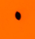
After examining individual BPE of various sizes and the effect of applied driving potential, we set out to study a linear array of interacting BPEs. The cell in this Chapter was fabricated using shadow mask (d) from Figure 2.4. The shadow mask also contained a triangular bipolar electrode. However, the triangular opening was blocked off, and only the linear array BPEs were studied here. With this shadow mask, a linear array of small disc BPEs with the same size and equal spacing was deposited between two driving electrodes. Utilizing the time-lapse fluorescence imaging technique, the doping from BPEs was captured and the propagation speeds were determined and compared. A simulation using COMSOL on the initial field distribution of the specific cell geometry was also performed. This simulation revealed the potential and electric field profiles of the cell and aided in the understanding of the observed cell behavior.

This code has a document (117 pages) which describe the algorithm in detail.

Inputs & Outputs :

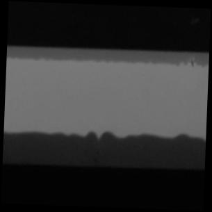
Conversion ratio: 0.01041 mm/pixel

Boundary y-ccordinate: 7.89 pixel

Boundary y-ccordinate: 70.87 pixel

Boundary y-ccordinate: 89.98 pixel

Boundary y-ccordinate: 193.35 pixel

MATLAB code for Doping Propagation in a Large Planar LEC

Planar LECs with a Linear Array of
Bipolar Electrodes

Conversion ratio: 0.00583 mm /pixel

Electrode Size(mm)         Confirm(mm)          Point1         Point2

0.1863                            0.1863                   (39, 57)          (69, 68)

0.1863                            0.1863                   (39, 57)            (69, 68)

0.1863 0.1863 (39, 57) (69, 68)

0.1863 0.1863 (39, 57) (69, 68)

0.1863 0.1863 (39, 57) (69, 68)

0.1863 0.1863 (39, 57) (69, 68)

0.1863 0.1863 (39, 57) (69, 68)

0.1863 0.1863 (39, 57) (69, 68)

https://matlab1.com/shop/matlab-code/matlab-code-doping-propagation-large-planar-lec/

https://qspace.library.queensu.ca/bitstream/1974/15155/1/Chen_Shulun_201610_Master.pdf