The Need for Speed in MRI
MR imaging speed is of critical importance in many clinical applications. However, the imaging speed with which gradient-encoded MR images can be acquired is fundamentally limited by the sequential nature of gradient-based MR acquisitions, in which only one k-space line can be acquired per unit time. In order to accelerate data acquisition, conventional MRI requires stronger field gradients, faster gradient switching rates, and/or more frequent RF excitations. Faster gradient switching can lead to peripheral nerve stimulation, and more frequent RF pulses can result in increased RF power deposition, with an increased risk of damaging biological tissues. Another way of accelerating MR imaging is to acquire reduced quantities of measurements without compromising image information or spatiotemporal resolution. Partial Fourier imaging is one of the simplest approaches for accelerated data acquisition in MRI. In this approach, approximately half of the k-space lines are acquired and the rest are estimated by exploiting the conjugate symmetry property of the Fourier transform for real-valued objects. However, the maximum acceleration factor in Partial Fourier imaging is limited to less than two. Parallel MRI, introduced in earnest in the late 1990s, is a more popular and more flexible approach for increasing imaging speed. Parallel MRI uses spatial information from an array of RF receiver coils to perform some portion of the spatial encoding that is normally accomplished via field gradients. Since signals in multiple receive coil elements may be acquired simultaneously, coil-based encoding enables acquisition of multiple lines of image data at the same time. Over the past two decades, parallel MRI has evolved rapidly, and it is implemented on most clinical MR scanners in use today. A generalized formulation of parallel MRI is briefly reviewed in this section.
Spatial Encoding Using Coil Arrays
In parallel MRI, an array of RF receiver coils is used for data acquisition. Each individual coil element has different spatially-varying sensitivities, as shown in Fig. 2.3. In the case of two dimensional
imaging, the k-space data acquired in each coil-element can be described by adapting Eq. (2.11) as follows:
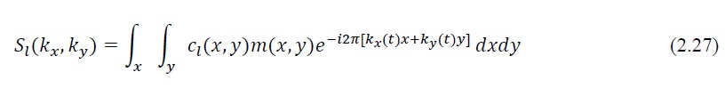

Fig. 2.3. An example of multicoil brain images with corresponding coil sensitivity maps with 6 coil elements. Each individual coil element has a different spatially-varying sensitivity pattern.
Here, l = 1,2,3, … , Nc is the coil index ( Nc is the total number of coil elements) and ?? (?, ?) is the coil sensitivity map for the l-th coil element. A hybrid encoding function can then be formulated as
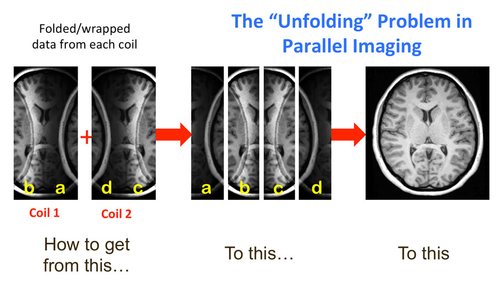
Equations (2.27) and (2.28) suggest that as long as the combination of different coil sensitivities can imitate the gradient encoding, some k-space lines that are traditionally acquired using gradient encoding can be generated retrospectively using the coil sensitivities. In other
words, the use of multiple receiver coils with different spatial sensitivities allows for acquisition of multiple k-space lines simultaneously.
Generalized Parallel MRI Reconstruction
The hybrid encoding function formulated in Eq. (2.28) does not form a pure Fourier basis, and thus reconstruction is more involved than an inverse Fourier transform. Combining Equations (2.27) and (2.28), we have
Or, with appropriate discretization
Eq. (2.30) can be rewritten in matrix notation as
Here vector s contains the measured multicoil MR signal (with size NcNk×1), m is the image vector to be reconstructed (with size N?×1), and E is the hybrid encoding matrix (with size NcNk×N?). It can be seen from Eq. (2.31) that theoretically the encoding matrix E remains
invertible as long as gradient encoding steps are reduced by no more than a maximum factor of Nc. In general, the reconstruction problem is over-determined, and thus reconstruction of image ?̂ may be performed by minimizing the mean square error
As is the case for Eq. (2.25), the solution of Eq. (2.32) can be found by computing the Moore-Penrose pseudoinverse
Here, the pseudoinverse has been generalized by including a noise covariance matrix Φ, which accounts for correlations in noise contributions from distinct array elements, and which can be computed from measurements in the absence of RF excitation (i.e. with a flip angle of zero). The noise covariance matrix is a practical tool to evaluate the noise distribution in different coil elements in the measurement system. The best reconstruction result can be obtained when any noise shared by more than one coil is removed from the problem. This step is commonly known as noise decorrelation or noise whitening.
Practical parallel MRI reconstruction methods are usually implemented based on particular sampling patterns (i.e., regular undersampling), or else using iterative reconstructions in the case of non-Cartesian sampling. Different parallel imaging techniques, such as SMASH, SENSE, and GRAPPA, have been extensively developed and broadly implemented for day-to-day clinical exams. The discussion of specific parallel imaging algorithms can be found in many classic papers and textbooks
Estimation of Coil Sensitivities
In parallel MRI, accurate coil sensitivity information is required in order to reconstruct the image from undersampled k-space data. Since the sensitivities can depend not only on the geometry of the coil array, but also on the object be imaged, estimation of coil sensitivities is
required for each individual scan. Additional reference data, which can be either acquired separately or self-calibrated, is used for coil sensitive estimation.
In parallel image reconstruction methods like SENSE, coil sensitivity maps must be calculated explicitly and then used to compute the encoding matrix so that the aliased image can be unfolded from undersampled measurements. In parallel image reconstruction methods like GRAPPA or SPIRiT , on the other hand, the coil sensitivity maps do not need to be calculated explicitly and the missing k-space lines are estimated using autocalibrated measurements acquired as an integral part of the data measurements. Autocalibration has the advantage that reconstructions are less sensitive to temporal changes such as motion. In dynamic imaging, the sampling pattern in different temporal frames can be specifically designed, so that the coil sensitivities can be estimated from the averaging of all the dynamic frames. In these methods, additional reference data is not necessary for coil sensitivities estimation. The raw sensitivity maps are generally corrupted by noise, and many approaches have been proposed to produce smooth sensitivity maps, such as the adaptive array combination.