MR Image Reconstruction
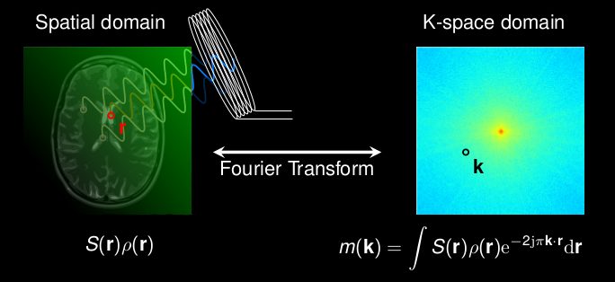
As shown in Eq. (2.11), MR signal from a two-dimensional plane is a spatial integration of the spin density against the sinusoidal spatial modulation generated by encoding gradients. In other words, the MR signal comprises projections of the spin density against Nx×Ny distinct functions, in which a total number of Nx×Ny measurements are obtained in the presence of frequency- and phase-encoding gradients. As discussed in the previous sections, appropriat discretization is needed in practical MRI acquisition and thus the integration in Eq. (2.11) can be approximated as
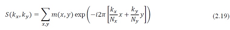
Eq. (2.19) represents the Fourier transform of the spin density in the two-dimensional plane with appropriate discretization of the continuous positions. Therefore, the reconstruction of the image can be formulated as the inverse discrete Fourier transform (DFT) of the MR measurements

The spatial encoding part in Eq. (2.20) can be written as
Eq. (2.21) is usually referred as “encoding function”, because it represents the way that spatial encoding is performed. Thus, Eq. (2.19) can be rewritten in matrix notation as
Here s is the measured MR signal vector in k-space (with size Nk×1), m is the image vector to be reconstructed (with size N?×1) and E is the encoding matrix that transforms the image vector into the signal vector (with size Nk×N?). Reconstruction of the image m is given by
inverting Eq. (2.22)
Supposing the measurement matrix E is full rank, the reconstruction described in Eq. (2.23) is discussed in three different situations.
i) When Nk=N?, the system is well-determined and then s can be uniquely reconstructed from Nk linearly independent measurements.
ii) When Nk>N?, the system is over-determined and, strictly speaking, there is no solution. In general, a good guess for the solution can be found by minimizing the mean square error
![]()
Here ‖∙‖2 is the L2-norm to quantify the energy or power of the difference between the measurements and the estimated solution. The solution of Eq. (2.24) is given by the Moore- Penrose pseudoinverse
Here H defines the Hermitian conjugate and ?̂ represents the approximate solution.
iii) When Nk<N?, the system is under-determined. This is usually the case for under sampling in MRI, and the solution is not unique. In this case, one classic way of arriving at a solution is to solve the following optimization problem :
Here ? is the estimated noise level. Based on the isometric property of the Fourier transform, minimization of energy in the image domain is equivalent to minimization of energy in k-space, and thus the solution to Eq. (2.26) is the zero-padded reconstruction, which can lead to aliasing artifacts in the result. Additional regularizations can be applied to reconstruct a better solution, which will be discussed more in the section on compressed sensing.