
Accelerating Parallel Image
Reconstruction Using Random Projection
Prologue
Random projection has been used for data dimension reduction . The concept of random projection is related to compressed sensing , a topic that has attracted many attentions recently. By projecting the data to lower dimensions using some random matrices with certain properties (e.g., the restricted isometry property), the useful information is still preserved in the reduced data
ntroduction
Parallel imaging using phased array coils has been widely used clinically to accelerate the MR data acquisition speed Generalized auto-calibrating partially parallel acquisition (GRAPPA) is a k-space based parallel image reconstruction method that has been widely used. It reconstructs the missing k-space data for each channel (known as the target channel) by a linear combination of some acquired data from all channels (source channel), where the coefficients for combination are estimated using some additionally acquired auto-calibration signal (ACS) lines. Massive array coils with a large number of channels have been studied and developed for higher signal-to-noise ratios (SNR) and/or higher accelerations . As massive array coils become commercially available, the greatly increased computational time has become a concern for GRAPPA reconstruction because the reconstruction time increases almost quadratically with the number of channels. Such a long reconstruction time using massive array coils leads to difficulties in online high-throughput display. A few works attempt to address this issue using hardware-based or software-based approaches to reduce the effective number of channels. In the hardware-based approach , a hardware RF signal combiner inline was placed between preamplification and the receiver system to construct an Eigencoil array based on the noise covariance of the receiver array. With such a channel reduction method, optimal signal to noise ratio (SNR) and similar reconstruction quality can be achieved. However, the requirement of additional hardware can be cumbersome. In contrast, it is more flexible to use the software-based channel reduction methods. The coil compression process generates a new set of fewer virtual channels that can be expressed as linear combinations of the physical channels. These methods aim at reducing the effective number of channels used for reconstruction by combining the physically acquired data from a large number of channels before image reconstruction. For example, principal component analysis (PCA) has been used to find the correlation among physical channels and reduce the number of channels to fewer effective ones by linearly combining the data from physical channels.These fewer combined channels are used for reconstruction, which leads to reduced reconstruction time. With channel reduction, both the numbers of target channels and source channels can be reduced. Since the ultimate goal is the reconstruction of a single-channel image, several studies have investigated to synthesize a single target channel for k-space-based reconstruction techniques. These methods compress multiple channels to a single channel prior to reconstruction so that the convolution-based calibration and synthesis only need to be performed once instead of for each channel and significant computation reduction can thereby be achieved.
Theory
Complexity of 2D GRAPPA
There are two phases in GRAPPA reconstruction, the calibration phase and the synthesis phase. During the calibration phase, the acquired ACS data is used to calibrate the GRAPPA reconstruction coefficients in k-space. Specifically, the k-space data point that should be skipped
during the accelerated scan is assumed to be approximately equal to a linear combination of the acquired under-sampled data in the neighborhood from all coils, which can be represented as
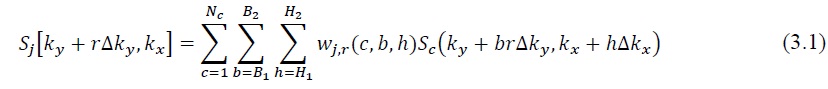
where Sj on the left-hand side denotes the target data that should be skipped but is acquired for the calibration purpose, and Sc on the right-hand side is the source k-space signals that should originally be acquired, both in the ACS region. Here w denotes the coefficient set, R represents the reduction factor (ORF), j is the target coil, r is the offset, c counts all coils, b and h transverse the acquired neighboring k-space data in ![]() and
and ![]() directions respectively, and the variables
directions respectively, and the variables![]() and
and ![]() represent the coordinates along the frequency- and phase-encoding directions, respectively. The GRAPPA calibration phase can be simplified as a matrix equation
represent the coordinates along the frequency- and phase-encoding directions, respectively. The GRAPPA calibration phase can be simplified as a matrix equation

where A represents the matrix comprised of the source data, b = [b1, b2,…, bl] denotes the target data for calibration, and x = [x1, x2,…, xl] represents the linear combination coefficients, l counts for all coils and all possible offsets and is equal to (R-1)Nc. A has rows and
columns, where Np is the number of phase-encoding lines that are possible fit locations, Nx is the number of points along the frequency encoding direction, Nc is the total number of all channels for the original k-space data, and dx and dy are the convolution size of GRAPPA along the frequency-encoding and phase-encoding directions respectively. The convolution size along the phase-encoding direction is defined as block size in GRAPPA. In general, the coefficients x depend on the coil sensitivities and are not known a priori. In calibration, the goal is to find the unknown x based on the matrix Eq. (3.2). The target data b and matrix A include data at all locations of the ACS region to find the best GRAPPA coefficients x. The least-squares method is commonly used to calculate the coefficients :
Many ACS data points are usually acquired to set up Eq. (3.2), which means the problem is well over-determined. In this case, the solution is given by :
![]()
During the synthesis phase, based on the shift-invariant assumption, the same Eq. (3.2) is used with the same x obtained from Eq. (3.4), but to obtain the unknown b using the acquired kspace data outside the ACS region for A. By this means, the missing data b is estimated by the linear combination of the acquired data in A and the full k-space data can be used to obtain the image of each channel. The final image is reconstructed using the root sum of squares of the images from all channels. The computational expense of the calibration and synthesis phases can be estimated using matrix multiplication and inversions . Several different distribution modes of the blocks can be used individually to estimate the missing data. These estimated data from different modes are then combined using the goodness of fit. For each mode, the calibration phase requires For each mode, the calibration phase requires +nl(m+n)+ complex-valued multiplications, where m = NpNx, n = dxdyNc, l = (R-1)Nc. It is seen that AHA dominates the calibration cost for m >> n, which requires complex-valued multiplications. Furthermore, in the synthesis phase of GRAPPA, ?????? 2???? (? − 1) complex-valued multiplications are needed for each mode, where Nu is the number of phaseencoding lines to be synthesized at a particular offset. The number of modes is commonly chosen to be the same as the number of blocks dy. The computation of the goodness of fit itself is typically negligible, compared to other calculations. Therefore, the total computational expense for GRAPPA reconstruction is approximately on the order of ???? (???? )2?? 3 + ?????? 2???? 2 (? − 1) + ?? 3?? 2?? 3 (? − 1) + (???? )3?? 4 + ?????? 2???? 2 (? − 1). The analysis shows that the computational complexity increases almost quadratically with the number of channels. Therefore, channel reduction methods are able to reduce the total reconstruction time significantly. On the other hand, the calibration phase is seen to involve high computational cost due to solving inverse equations. If we adopt the commonly used reconstruction parameters = 30, ![]() = 256, dx = 13, dy = 4, R = 3,
= 256, dx = 13, dy = 4, R = 3, ![]() = 75,
= 75, ![]() = 8, block size = 4,
= 8, block size = 4, ![]() =24, the ratio between the calibration and synthesis phases is 9.3. This confirms the calibration process dominates the total computational time
=24, the ratio between the calibration and synthesis phases is 9.3. This confirms the calibration process dominates the total computational time
PCA based Dimension Reduction Method for Channel Compression
Dimensionality reduction has been well studied in the machine learning community. It involves projecting data from a high-dimensional space to a lower-dimensional one without a significant loss of information. The new data with reduced dimensions is expected to maintain most important information. Among the existing linear approaches which use linear mapping for the dimensionality reduction, PCA is a classical method to remove redundant information from statistically correlated data and reduce the dimensions. It performs the eigen-decomposition on the covariance matrix of the data and removes the components that correspond to the smallest eigenvalues. Among all linear approaches, PCA minimizes the projection residuals and maximizes the variance between the combined variables . A major limitation of PCA is its computational complexity. Performing a PCA requires an order of N3 multiplications with N being the original dimension, which becomes prohibitive when dealing with a large dataset. In parallel imaging, PCA has been successfully used to compress the channels in large array coils . The resulting fewer combined channels corresponding to the largest eigenvalues are used for reconstruction such that the reconstruction time is reduced. Because the number of channels is not a large number in general, the computational saving from channel reduction overrides the additional computational cost of PCA.