Bayesian Statistics

A hypothesis is nothing more than a claim or premise that one is interested in verifying. In imaging and spectroscopy, one example is that at a certain location in the eld of view, the hypothesis is that a spectrum is present. Another hypothesis is that the mean value of the signal is some value. Often times one is interested in estimating parameters of stochastic processes, which we denote $\theta$ . Bayesian statistics allows one to treat the hypothesis or parameters as random variables rather than deterministic constants. At the heart of Bayesian approaches is Bayes’ theorem, which is a way of computing probabilities of a hypothesis give some evidence which are related to the hypothesis. The idea is that one can make

a more informed calculation of probability if one is able to update the probability given some new piece of evidence that one may have not had at the beginning. The derivation of Bayes’ theorem follows from the denition of conditional probability. The conditional probability of event A occurring given that B occurred is :

this can be seen graphically in Figure 2.2. Solving for the joint probability $P$ $(A\bigcap {}B)$ gives

since the joint probability commutes $P$ $(A\bigcap {B})$ $=$ $P$ $(B\bigcap A)$ , we can also write

equating the right hand sides of Equation 2.19 and Equation 2.20 gives use Bayes’ theorem (also called Bayes’ rule)

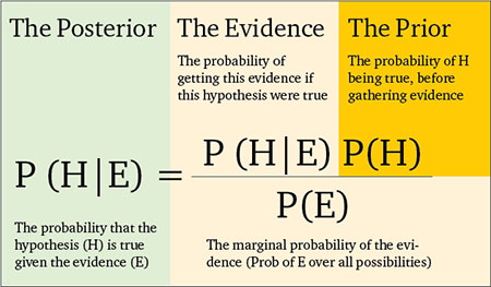
One interpretation of Bayes’ theorem is called the Diachronic interpretation, which says that conditional probability of the hypothesis or parameter given knowledge of some evidence or measurement data is given by

The term $P(\theta|g)$ is called the posterior . It represents the belief in the hypothesis given the data. The term P ( $\theta$ ) is called the prior . $P(\theta|g)$ is called the likelihood. P ( $\theta$ ) is called the normalizing constant, which is computed to ensure that the posterior probabilities sum to 1. The normalizing constant can be written as

One can repeatedly apply Bayes’ theorem given new measurement data.

Example : Updating Probabilities with Bayes’ Theo-rem

I will use a simple example to illustrate how to update probabilities using Bayes’ theorem, see Figure 2.3. Imagine I have two bags of candy, Bag 1, which I denote $B_1$ , and Bag 2, which I denote $B_2$ . Bag 1 has 10 pieces of cherry avored candy,At the beginning, the prior probability of selecting bag 1 or bag 2 is both equal

Someone then picks a bag at random and takes out a piece of candy that turns out to be strawberry avor. They do not state which bag was selected, only that the candy they randomly selected from the bag was strawberry. What is the probability that bag 1 was the one selected given that I know the candy is strawberry? I can use Bayes’ theorem to compute this

$P(S|B_1)$ is the probability of selecting strawberry given that they pick bag 1, which is 3=4. P (S) is the probability of selecting a strawberry candy from either bag 1 or bag 2, which 5/8. Thus Now to continue the example. Imagine the First piece of candy is put back into the bag from where it came from. Then another piece of candy is drawn from the same bag, which turns out to be cherry avor. Now one must update the probabilities with this new piece of information. One can keep using Bayes’ theorem. The posteriors from the last draw m – 1 are now used as the priors for the current update.

The probability of drawing a cherry avored candy assuming bag 1 was chosen
remains constant since the ratio of cherry to strawberry did not change for either
bag, so $P(C|B_1)=1/4$ and the probability of drawing a cherry avored candy assuming bag 2 was chosen is 1/2. We now must use Equation 2.23 to compute the normalizing constant, otherwise the posterior probabilities will not sum to 1. In this case P(C)= 7/20. Plugging these numbers into Equations 2.27 and 2.28 gives the updated posterior probabilities

Intuitively, drawing a cherry avored candy has reduced our belief that bag 1 was chosen since bag 1 consist of only 1/4 cherry avor candy while bag 2 consisted of 1/2 cherry candy. This sequence can be continued, until a threshold has been reached for one of the posterior probabilities.

Maximum A Posteriori

Imagine a situation similar to the candy example, where we are given a set of hypotheses, $\left \{ h_1,h2,...h_N_R \right \}$ , and we are interested in nding which hypothesis is the most likely, after new measurement gm is made. The method of Maximum A Posteriori (MAP) says the hypothesis $h_k$ which maximizes the posterior probability is the most likely one.

Using Bayes’ theorem I can rewrite Equation 2.31 as

Maximizing the posterior is now equal to maximizing the likelihood and prior. In certain cases, one needs to decide between two sets of parameters or hypotheses. One can do an analogous technique of comparing the posteriors by using a ratio

If the ratio is larger than some threshold value then one choses parameter $h_i$ and if the ratio is less than the threshold then one choses $h_j$ . Similar to the earlier example of updating the posterior based on new data, one can update the Maximum A Posteriori (MAP) decision based on new data. Dene the likelihood ratio of the $m ^{th}$ measurement as

After each new set of measurement data $g_m$ is collected, one can update the posterior ratios by multiplying the likelihood ratio from the old set of data with the likelihood ratio of the new set of data. The ratio which includes all the updates from measurement m = 1 to measurement m = $N_m$ is written as

where the notation $\left \{ g \right \}N_m$ represents the set of all data from measurement $m$ to $N_m$ . In summary, Bayesian statistics is a useful way to update one’s belief in a hypothesis or estimate a set of parameters. Bayes’ theorem can be used to merge new measurement data and the probability of a hypothesis before the data was known. This is very similar the approach taken by the Adaptive Feature Specic Spectrometer (AFSS) and the AFSSI-C

https://search.proquest.com/openview/4c390c5e298854ed9383815aca5431c0/1?pq-origsite=gscholar&cbl=18750&diss=y

Bayesian Statistics