Ultrasonic Communications in Human Tissues

Fundamentals of UltrasoundWaves

Ultrasounds are mechanical pressure waves with a frequency above the upper limit of human hearing, i.e., 20 kHz. Ultrasounds consist of mechanical vibrations of particles in a material. Even if each particle oscillates around its rest position, the vibration energy propagates as a wave traveling from particle to particle through the material. Acoustic waves in general can be characterized by their physical parameters as follows:

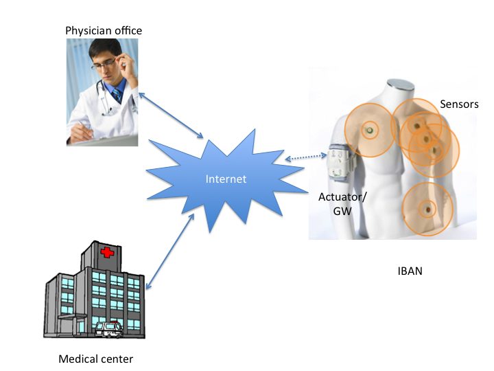
Figure 1: System architecture

• The frequency, f, represents the number of complete oscillations per second for each particle. As stated above, ultrasound waves have a lower bound of 20 kHz.
• The pressure, P, is a measure of the compressions and rarefactions of the molecules in the medium through which sound waves propagate, and is typically measured in Pascal [N/m2].
• The amplitude, A, represents the displacement of particles from their rest position. • The propagation speed c is the rate at which the vibratory energy is transmitted in the direction of propagation and increase with the rigidity of the material. In tissues, we consider an average sound speed of 1540 m/s.
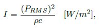
• The intensity, I, is the average energy carried over time by a wave per unit area normal to the direction of propagation and is usually measured in mW/cm2. It can be expressed as a quadratic function of pressure as

where PRMS is the sound pressure root mean square (rms), ⇢ and c represent the density of the medium and the speed of sound in the medium, respectively.

Attenuation

When ultrasound waves propagate through an absorbing medium, the initial pressure, $P_0$ reduces at P(d) at a distance d according to

Figure 2: Attenuation in the blood as a function of the operating frequency for different values of distance.

where $\al$ (in [np · $cm^{-1}$ ) is the amplitude attenuation coefficient that captures all the effects that cause a dissipation of energy from the ultrasound beam. This parameter $\al$ is a function of the carrier frequency as

where f represents the carrier frequency and a (in [np $m^{-1}$ $MHz^{-b}$ ]) and b are attenuation parameters characterizing the tissue. Typical experimental values of these parameters in different tissues are reported in Table 2.
Based on this, we can compute and plot attenuation as a function of propagation frequency for different

Table 1: Tissues parameters

mediums. Results for blood are reported in Fig. 2.
Since most sensing applications require highly directional transducers, one needs to operate at high frequencies to keep the transducer size small. Conversely, as shown in Fig. 2, higher transmission frequencies lead to higher attenuation. Therefore, for effective ultrasonic communications we need to operate at frequencies compatible with small devices, but at the same time limit the maximum attenuation. In Fig. 3, we depict the maximum carrier frequency with respect to the distance, for different maximum attenuation values, assuming blood as the propagation medium, and limiting the maximum operating frequency to 1 GHz. Table 3 ummarizes our results for a 100 dB attenuation. Since the attenuation increases as a function of frequency

Figure 3: Maximum Carrier Frequency in the blood.

and distance, for a fixed value of attenuation we get an inverse relationship between frequency and distance. For communication distances that range from some μm up to a few mm (what we refer to as short-range communications) frequencies higher than 1 GHz are allowed. When distances are larger than 1mmbut still lower than some cm, i.e., for medium range communications, transmission frequencies should be decreased to approximately 100 MHz. For distances higher than a few cm, i.e., for long range communications, the transmission frequency should not exceed 10MHz.

Table 2: Frequency Limits for A=100 dB

Ultrasonic Transducers

To accurately model the ultrasonic communication channel in tissues we need to understand how propagation parameters are affected by the characteristics of the transmitting and receiving devices. An ultrasonic transducer is a device capable of generating and receiving ultrasonic waves. It is primarely made up of an active element, a backing, and a wear plate. The active element is usually a piezoelectric material that converts electrical energy to ultrasonic energy and vice versa. The backing is a very dense material used to absorb the energy radiated from the back face of the piezoelectric element. The wear plate allows to protect the piezoelectric transducer element from the environment and is selected to protect against wear and corrosion.
The acoustic radiation pattern of a transducer is a representation of the transducer sound pressure level as a function of the spatial angle and is related to parameters such as the carrier frequency, size, and shape of the

Figure 4: Minimum transducer diameter as a function of the operating frequency.

vibrating surface. Furthermore, the acoustic radiation pattern is reciprocal, i.e., its shape is the same whether the transducer is working as a transmitter or as a receiver. Depending on the desired application, transducers can be designed to radiate sound according to different patterns, e.g., omnidirectional or in very narrow beams.
For a transducer with a circular radiating surface, the narrowness of the beam pattern is a function of the ratio of the diameter of the radiating surface and the wavelength at the operating frequency, D/ $\lam$ . This relationship can be explained by considering the beam spread formulas defined as

where $\al/2$ is half the angle spread between the -6 dB points. The higher the frequency or, the larger the transducer’s diameter, the smaller the beam spread. In Fig. 2.4, we show the minimum diameter of the transducer for different values of $\al$ as a function of the operating frequency. When a transducer is working as a transmitter, it is usually characterized in terms of pressure level. In particular, the sound pressure level [ind B referred to μPa] is defined as:

where $P_{RMS}$ [μPa] is the sound pressure rms and $P_{REF}$ is the reference pressure, equal to 1μPa in underwater environments. This pressure value can be converted to intensity through eq. (2.1), assuming appropriate values for density and speed of sound in tissues. The main parameter characterizing a transducer used as a receiver of acoustic signals is the sensitivity (Sen) [dB re V/μPa], which can be defined as the voltage output found at the receiver when a specific value of SPL is given, i.e.,

Figure 5: Voltage Output vs. SPL Input, assuming different sensitivity values.

where $V_{SPL}$ is the output voltage given by a specific SPL value. In Fig. 5, the I/O relationship for transducers with different sensitivity values are reported. These plots show the output in Volts, given an SPL value in dB re μPa, for different sensitivities expressed in dB re Volt/μPa.

Reflections and Scattering

Whenever a sound beam encounters a boundary between two materials, some of the energy is reflected, thus reducing the amount of energy that passes through that boundary. The direction and magnitude of the reflected and refracted wave depend on the orientation of the boundary surface and the difference between the different tissues. This mirror-like reflection can be expressed using the Snell law for acoustics.
When an acoustic wave encounters an object that is relatively small compared to the wavelength, or tissue with an irregular surface, a phenomenon called scattered reflection occurs. To describe scattered ultrasonic waves we need to model the statistics of the signal in a very general environment. Therefore, the model must have parameters that take in account tissue characteristics and are simple to compute. A model that satisfies these requirements is based on the Nakagami distribution.
If we consider a transmitted signal s(t), the received signal due to scattering effect, assuming a noiseless channel and non-selective slow fading, can be expressed as

To characterize the statistical behavior of the received signal, we assume the phase shift $\phi$ to be uniformly distributed in [0, 2 $\pi$ ] and the magnitude $\rho$ to be Nakagami-distributed. Therefore, the probability density functions of these random variables are expressed as

where m is the Nakagami parameter, $\Ome$ is a scaling parameter, U(·) is the unit-step function, $\Gamma$ (·) is the gamma function, and $rect_{2\pi}$ (·) is the rectangular function of duration $2\pi$ . Varying the value of the Nakagami parameter, we obtain different distributions such as the Gaussian distribution (m = 0.5), the Rayleigh distribution (m = 1) and the Rician distribution (m > 1). Therefore, the Nakagami amplitude distribution can describe different scenarios simply varying the value of m.
Since the human body is composed of different organs and tissues, each of them with different sizes, densities, and speed of sound, it can be modeled as an environment with a pervasive presence of reflectors and scatterers. Consequently, the received signal is obtained as the sum of numerous attenuated and delayed versions of the transmitted signal, which makes propagation in ultrasonic intra-body networks deeply affected by multipath fading.

Noise Sources

No previous study, to the best of our knowledge, has investigated in detail noise sources in tissue propagation. In underwater communications, the ambient noise level is given by the intensity of the ambient noise, expressed in dB re μPa, and is usually expressed as a sum of different components. Since we are focusing on ultrasonic frequencies, we focus on the thermal noise produced by the agitation of molecules in tissue. As in, the power spectral density (PSD) of the thermal noise obtained for an ideal medium using classical statistical mechanics can be adopted with good approximation for a real medium such as body tissues.
Assuming different densities and sound speed for the medium, we can derive an expression for the noise PSD in dB re μPa per Hz as

with f expressed in kHz. Based on (2.10), we can express the system SNR as

where P is the transmitted power, N(f) is the PSD of the noise, assumed to be equal to the PSD of the thermal noise, and A(d, f) is the attenuation experienced by the transmitted pressure signal. From eq. (2.2), A(d, f) can be expressed as

To estimate the impact of frequency and distance on the SNR, we can focus on the expression of (A(d, f)N $(f)^{-1}$ only. This quantity is shown in Fig. 6 as a function of the transmission frequency, assuming blood as the propagation medium and considering different propagation distances. Since noise and attenuation are monotonically increasing functions of the operating frequency, (A(d, f)N $(f))^{-1}$ monotonically decreases with increasing frequency. Furthermore, since attenuation is also a function of the propagation distance, our results show that (A(d, f)N $(f))^{-1}$ decreases faster as the link distance increases.

Figure 6: (A(d, f)N(f))−1 when the propagation medium is blood

Bandwidth Evaluation

Based on this discussion, we can make some preliminary considerations on the bandwidth available for ultrasound communications in tissues. As in, we maximize the channel capacity using an optimal energy allocation for a fixed transmission power.
When we maximize the capacity with respect to the power spectral density of the signal denoted as $S_d(f)$ , assuming a finite transmission power P, we obtain an optimal power distribution, and the solution satisfies the water-filling principle:

where $K_d$ is a constant depending on the value of P, which is fixed according to the desired SNR value. Therefore, to achieve maximum capacity through an optimal energy allocation, the total PSD on the channel’s band has to be flat and equal to $K_d$ . The maximum capacity obtained can be expressed as in

where B(d) is the bandwidth that varies depending on the distance d. Assuming now the desired SNR equal to 20 dB, we can compute the desired bandwidth and the maximum capacity using the numerical procedure reported in. In Fig. 7 bandwidth and capacity are shown as a function of the propagation distance. In this plot, we assume 1 GHz, 100 MHz and 10 MHz as operating frequencies for the short-, medium- and long-range communications, respectively, Using the appropriate operating frequencies as identified in Table 3, the bandwidth and capacity decrease almost linearly in log-scale as distance increases. This shows that high data rates can be reached in case of long distance communications, which provides a strong motivation for seeking to achieve robust and reliable communications through high-bandwidth signaling techniques such as ultra wide band (UWB) and/or code division multiple access (CDMA).

Figure 7: Bandwidth [Mbit/s] and Capacity [MHz] vs. propagation distance.

Ultrasonic Communications in Human Tissues