Spike Detection Units and Setup

Integration of Several Spike Detection Units:

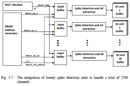
The total number of channels to be processed is reconfigurable. According to the neural signal processing algorithm used, the longest process applied after sample reading was to copy the first 16 samples of an AP. This procedure required nineteen clock cycles. To have an optimum hardware usage, twenty spike-based reduction units were integrated, so that channels on other units can be updated with their respective sample inputs while this longest procedure is being completed, and before that same unit receives a new incoming sample. 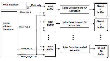Fig.1 presents the initial integration of twenty spike detection units to handle a total of 2560 channels.

Addressing and Timing:

The BRAM assignment has been chosen so that the BRAM_address can provide direct information on the channel order on the input BRAM and the sample number as shown in Fig.2. The write address generator constructs the BRAM write address to rearrange the sample data in preparation for a structured processing. It concatenates the output of three counters to write each sample data in the corresponding channel location.
The BRAM address generator operates at a frequency f, where:
f = sampling frequency per channel x number of channels
For the example of integrating twenty SD units, the BRAM address concatenates the output of three counters:
(a) a 5-bit counter presenting the Input BRAM ID (20 input BRAMs)
(b) a 7-bit counter presenting the channel order on the BRAM (128 channels per BRAM)
(c) a 4-bit counter presenting the sample number. (16-sample space per channel)
Counter (a) is the fastest changing at every clock cycle. Counter (b) is incremented after (a) reaches a full count cycle of 20 and then is reset. Counter (c) is the slowest counter, that only increments at the full count of counter (b).

Transmitting the APs from the Output Buffers to a Host PC:

The design structure can be extended to integrate spike sorting blocks. In this case the spike sorter will be reading the AP waveforms from the output buffers in their complete format. The dissertation work does not include a spike sorter, and the AP waveforms were sent to a host PC for system evaluation. The data were transmitted using PCI express (Peripheral Component Interconnect express) to a host PC. The data transmission performance was closely examined to make sure that the transmission latencies meet the system requirements and that there is enough hardware resources to cover the expected transmission queue depths. The system was tested for performance integrity assuring that no data was dropped.
Real-time hardware-implemented neuronal spike-based data reduction schemes are an attractive method to alleviate the bandwidth requirements for raw data transmission, and to increase the data acquisition throughput. The idea of data reduction was to send only the spike waveforms while disregarding the inter-spike samples. The spike waveforms are the only information needed for successive spike sorting. Based on the sparse nature of the neural signal with respect to time, and the average neuron firing rates, the amount of sent data can be reduced to approximately ~2.25% of the total amount of raw data.
The transmission from several output buffers corresponding to multiple Spike Detection units required the use of an intermediate FIFO to copy the AP waveforms to before transmission to the host PC. The copying process from multiple buffers was scheduled using queuing based control.

Transmission Latencies:

With a focus on telemetry transmission, Bossetti et al raised an important design consideration for spike-based data reduction in real-time. It was demonstrated that although the spike-based compression might be very appealing from the point of view of average bandwidth, it is subject to transmission bottlenecks during periods of multichannel neuron bursting causing queuing-based delays at the output buffer. They drew the attention to the relation between the ratio of the output to average input bandwidth and transmission latency, the number of samples per spike waveform, the mean firing rate MFR, and the needed queue depth of the output buffer memory. Bottlenecks and latencies are mainly a consequence of accumulating the input data samples over short periods of time before their transmission at the output. Based on statistical data performed on a 32-neuron system with an average neuron firing rate of 8.93 spikes/s, it was concluded that the output bandwidth had to be 3-5 times the overall average input firing rate to reduce the average maximum delays to less than the recommended limits of 10ms.
The model that they used relied on finding the average Firing Rates FR over 1ms time intervals and calculating the corresponding accumulation of AP waveforms in the output queue at different transmission rates. Their model neglected the reading and writing delays and assumed that the spikes were sent in bulk to the output FIFO. It was worth investigating if their model based on 32-neurons can be applied with the same binning parameters can be applied on a high-channel count system, and if the same transmission to FR ratio requirements would still apply to limit transmission latencies.

Overview on Bursting:

Burst is a term used in literature to describe a neuron’s firing in a clustered pattern. Each such burst is followed by a period of quiescence. Burst synchronization refers to the alignment of bursting and quiescent periods in interconnected neurons. Burst synchronization is the phenomenon that causes the longest queuing based transmission delays. Neocortical neurons can be classified into different types according to their pattern of spiking and bursting. All excitatory cortical cells are divided into three main classes as shown in Fig 3 and they are: Regular Spiking (RS) neurons, intrinsically bursting (IB) neurons and chattering (CH) neurons.

• • Regular Spiking (RS) neurons:

RS neurons are the most commonly encountered neurons in the cortex. When stimulated at threshold, an RS neuron generates only one spike. As the stimulus amplitude increases, the neurons respond with an initial high-frequency spike output, then they exhibit obvious frequency adaptation. A neuron might produce clusters of spikes in response to synaptic input. Some literature have reported a starting frequency spike output response of 320Hz, which declined to a much lower sustained frequency (< 100 Hz) within less than 50msec.

• • Intrinsically Bursting (IB) neurons:

IB neurons fire a stereotypical burst followed by repetitive spikes. Bursts are often the minimal response to a threshold stimulus. A burst can consist of few spikes firing at high frequencies in the range of 300 Hz and then followed by individual spikes firing at 15-20 Hz.

• • Chattering (CH) neurons:

CH neurons can generate rhythmic stereotypical bursts of closely spaced spikes. The typical inter-burst frequency is in the range of 5-15 Hz but can also be as high as 40 Hz.
In general, if a network of bursting neurons is linked, it will eventually synchronize for most types of bursting. Synchronization can also appear in circuits containing no intrinsically bursting neurons; however its appearance and stability improves if the network includes intrinsically bursting cells. Some literature described multichannel bursting as Neuronal Avalanches. Spiking activity propagates as individual neurons trigger action potential firing in subsequent neurons. They initiate a cascade that spreads through the neuronal network.

Super-Bursting:

High frequency network-wide bursting has been reported in research monitoring neural activity using MEA. This “super-bursting” was documented as a phenomenon of early plasticity that is ultimately refined into mature stable neural network behavior. Developmental super-bursting is thought to accompany transient states of heightened plasticity both in culture preparations as well as across brain regions.

A Model to estimate the required Transmission Rate:

Designing a platform that should handle hundreds to a few thousands of recording channels, it was essential to test if the output/input bandwidth ratio values recommended by previous literature, based on a limited number of monitored neurons, holds for a larger number of neurons. A transmission model was created in MATLAB to carry out simulations on the neuronal activity recordings of 2550 channels over 2.5 seconds. The model was constructed to detect spikes using the NEO operator. The threshold was set at 10 times the mean deviation over the complete 2.5 seconds of recording time. Each channel was handled separately and the spike times were saved.
Then simulations were carried out using a windowing format. In this case, spikes across the 2550 channels were collected over a 1 milliseconds period, rounding the recorded spike times to the nearest 1 millisecond. The queue depth based on the estimated transmission rate was found along the recording time. The spike times and transmission rate were used to calculate maximum latencies and queue depths.
At each rounded spike time, the corresponding detected spikes were added to the queue. The transmission rate determined how much of that data could be transmitted before the next load of binned spikes arrived, as well as the time required to remove the data from the queue. If spikes arrived before the queue was empty, the new data was added to the queue, increasing its depth. Latency was calculated from the queue size and represented the total amount of time required to remove all of the data from the queue at the estimated transmission rate. Following the recommended ranges of bandwidth ratios, the average firing rate was measured for the recorded data set used for testing and the transmission rate was set to be 5 times the MFR.

Data sets used for testing:

To test the model four in vitro data sets were used. The neural signals recorded using high-density MEA from 3Brain (www.3Brain.com) have been supplied by the NetS3 Lab in the Neuroscience Department of the Instituto Italiano di Tecnologia (IIT), Italy. Two sets were recorded using dissociated rat hippocampal cells (22 days in vitro) and two sets were taken from rat cortical cultures (21 days in vitro). The hippocampal and cortical neurons have a different dynamic firing pattern that was interesting to observe and analyze using this model (Fig 4-7). The hippocampal neurons tend to have a more synchronized firing behavior showing clear bursting events followed by relatively silent intervals. It was expected that they may represent a more critical case for the designed model in terms of the queue depths. The cortical neurons tend to be less synchronous and more spread from a spatial point of view. The validation of the model on cortical neurons was important since they are the mostly recorded type of neurons especially in vivo.