Description
In this Online Courses, you will learn how to implement optical flow in MATLAB.
Optical Flow MATLAB computer vision
In recent years, the optical flow has found many applications in machine vision.
In general, obvious motion changes in the brightness of an image are said to be due to the movement of targets. However, changes in the intensity of motion are similar to changes in ambient light or shadow but do not include optical flow.
The shorter the time between taking two consecutive images, the more similar the images are to each other, in which case the changes can be displayed in vector format proportional to the speed of the image coordinate device. In this case, the movement of the camera between the images is equal to the speed and the changes in the image mapping the speed of the environment. This small motion in the image is called optical flow.

Optical flow is usually considered in two ways, in the dense state, where the flow vector is calculated for each pixel, and in the feature-based state, which is calculated for the specific purposes for which it is intended.
If we want to calculate optical flow in a spherical model, we must either the first sample the environment as spherical space and then calculate optical flow (which is difficult and requires a lot of calculations), or optical flow is calculated in ordinary space and the result is through The Jacobin matrix is transferred to the spherical space.
Content title:
How many frames are needed to calculate Optical flow?
Example of a Hamburg taxi and the corresponding optical flow image
Example 2 Optical flow image
Example 3 Optical flow image
Example 4 (garden dataset) and the optical flow image
In which areas of the image, the optical flow faces a problem?
Display sample video and optical flow vectors on it
Examine situations in the video where the optical flow gives a bad result?
The distance and proximity of the object to the camera and its effect on optical flow
The difference between the light intensity of the object and the background and its effect on the calculation of optical flow
What is the main idea in optical flow?
Mathematical relations of the main idea of optical flow
The difference between motion and optical flow
Is every motion an optical flow?
Impact of lightening on the calculation of optical flow
When does Lucas-Kanade make a mistake?
When does Keypoint Mataching enter the optical flow calculation?
When does Region-Based matching enter the optical flow calculation?
When does the Gradient Constant enter the optical flow calculation?
Start MATLAB optical flow programming
OpticalFlow command
the MATLAB program draws a random optical flow
The concept of optical flow numbers
Draw optical flow vectors
DecimationFactor option
ScaleFactor option
OpticalFlowHS command
The second MATLAB program
Read video file
Explain the output parameters of the video reading command
Calculation of the frame width
Calculation of the frame height
Calculation of the total video frames
HasFrame command
ReadFrame command
EstimateFlow command
Optical flow output fields
Concepts Vx, Vy, Orientation and Magnitude
Calculate the minimum and maximum optical flow size
View optical flow on the video frame
Place a condition on the size of the optical flow
Morphological operation on the image
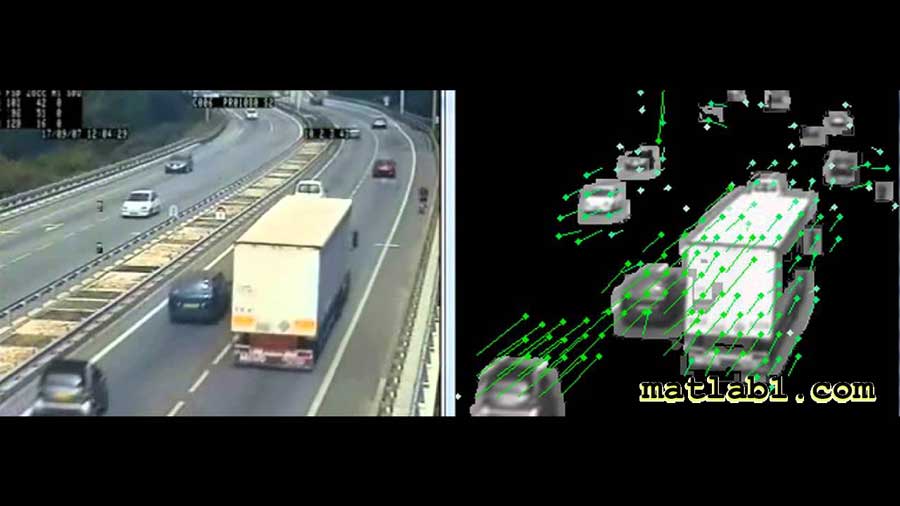
Object tracking based on optical flow
Place the bounding box on moving objects
InsertShape command
Smoothness parameter
MaxIteration parameter
VelocityDifference parameter
What are the conditions for stopping optical flow?
How to control the stop conditions?
Impact of each parameter in an example MATLAB application
The opticalFlowLK command
NoiseThreshold option
The Lucas-kanade method is a derivative of the Gaussian method
The opticalFlowLKDoG command
NumFrames option
ImageFilterSigma option
GradientFilterSigma option
NoiseThreshold option
Why is it better to use multiple frames in the optical flow calculation?
Reviews
There are no reviews yet.