
introduction
Glaucoma is one of the leading causes of signicant vision loss and blindness through- out the world. The disease is characteristically dened as a chronic optic neu- ropathy that results in the loss of retinal ganglion cells and their axons (i.e. the retinal nerve ber layer; RNFL), with increased intraocular pressure being the pri- mary risk factor. It is the cumulative loss of these retinal ganglion cells that leads to permanent visual eld defects and eventual blindness. Thus, the goal of clinicians is to detect glaucoma as early as possible in the disease process in order to preserve visual function. New advances in technology have resulted in the development of quicker, high- denition spectral-domain optical coherence tomography (SD-OCT) imaging with a retinal image resolution of 3:9m. Glaucoma analysis software has been developed to examine for glaucomatous retinal defects by identifying macular retinal thickness and asymmetry between the superior and inferior hemields. Total retinal thick-ness is calculated as the distance between the inner-limiting membrane (ILM), lying on the interface between the dark vitreous environment and the bright RNFL, and the highly re ective retinal pigmented epithelium (RPE), the last clear boundary between the retina and the vessels of the choroid (Fig. 1.1(a)).
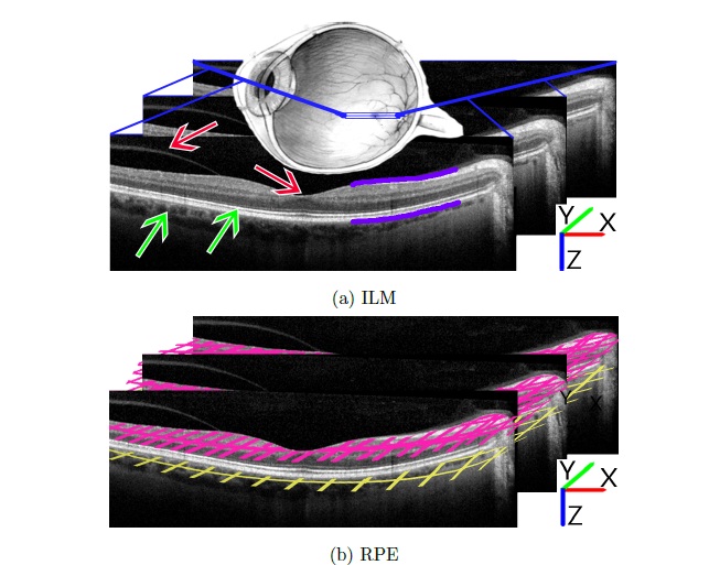
Figure 1.1.: Three sequential images taken from within an SD-OCT image stack of the human retina. Note Cartesian axes for future reference. (a) Purple lines denote the two layers of interest to be segmented: inner-limiting membrane (ILM) above, retinal pigmented epithelium (RPE) below. In a completely segmented image, the lines would extend along the layers in both directions. Red arrows indicate potential difficulties for the ILM: vitreous artifact at left presents an area of continuous contrast similar to the ILM; topological dip at the foveola is often accompanied by a reduction in absolute contrast, making a concrete measure of contrast impractical. Green arrows indicate potential issues for the RPE: both the choroid (left) and inner/outer photoreceptor segment junction provide areas of contrast similar to that of the RPE. (b) Two lightly- colored grids demonstrate the nal desired result for a 3D segmentation of the two layers.
Segmentation of OCT Scans using Deformable Models
The realm of deformable models can be divided into two classes: the implicit/geometric models and the parametric models. Currently, only a few deformable model ap-proaches have been presented to segment various aspects of OCT images, and all belong to the parametric model category, including that explained in this article. In 2005, Cabrera Fernandez rst demonstrated the utility of parametric deformable models through demonstration of the accurate segmentation of the uid-lled regions common in the OCT’s of patients with age-related macular degeneration. That same year, Mujat investigated a deformable model using splines for retinal layer segmentation, but limited their analysis of a 3D SD-OCT image stack to se-quential 2D analysis of the images. Few details of the proposed method were published, and it is difficult determine the relatedness of the algorithm to that demonstrated here due to a dearth of information. Total segmentation time for a stack using Mujat’s method was given as 62 seconds. In 2009, Mishra et al developed an algorithm with a basis in active contours to segment multiple layers in the re- sults of time-domain OCT, a precursor of the signicantly higher resolution SD-OCT technology . Reported segmentation time was considered \highly ecient” at ve seconds per 2D image, also known technically in the world of ophthalmology as a B-scan.
Highest Condence First
The HCF algorithm was originally presented by Chou et al. in 1990 as an \efficient”, \predictable”, and \robust” edge-detection algorithm for 2D images using a Markov Random Field (MRF). It has since been used across the computer vision community for various segmentation tasks including object segmentation in both 2D and 3D images, object tracking in video sequences, and text and handwrit-ing identication . HCF operates on an arbitrarily shaped MRF, a structure
generally composed of a layer of interconnected nodes. Each of these is connected to an additional node that is a representation of a random variable at the connected node’s location. This is the label for the connected node.
http://docs.lib.purdue.edu/dissertations/AAI1599021/
