Review of Magnetic Resonance Imaging (MRI)
The hydrogen atom has a nucleus consisting of only a single proton. Because of this it exhibits a relatively large magnetic moment. Hydrogen is also plentiful throughout the body due to its presence in every water molecule (). These properties make it a robust imaging target for MRI, although other nuclei can also produce images (e.g., Fluorine). In the presence of an external magnetic field a torque is applied to the magnetic moment (“spin”) of protons causing them to rotate into alignment with the direction of the field. The spins may align either parallel to the field, which is a stable low energy state; or anti-parallel to the field, which is a high-energy unstable state. The ratio of parallel to anti-parallel spins is given via the Boltzmann distribution:
Where k is the Boltzmann constant, T is the temperature, and ΔE = ħγ![]() . For a field strength of 3T at room temperature the equation reveals that only about 1 / 100,000 spins will be in the parallel state. This slight excess produces a net magnetic moment aligned in the direction of the applied field. This is known as the longitudinal magnetization and is given the symbol
. For a field strength of 3T at room temperature the equation reveals that only about 1 / 100,000 spins will be in the parallel state. This slight excess produces a net magnetic moment aligned in the direction of the applied field. This is known as the longitudinal magnetization and is given the symbol ![]() . Additionally, the torque applied to the spins by the external field causes them to precess at a specific frequency, described by the Larmor Equation:
. Additionally, the torque applied to the spins by the external field causes them to precess at a specific frequency, described by the Larmor Equation:
1
Here, γ is the gyromagnetic ratio and ![]() is the external field strength. For hydrogen γ = 42.58 MHz/T. In a 3T magnetic field, the resulting Larmor frequency for protons is 127.74 MHz. The longitudinal magnetization alone cannot produce a detectable signal as it does not vary with time. However, by inducing precession of the longitudinal magnetization it is possible to generate a time-varying magnetic field that lies in the transverse plane. This is accomplished by the application of an additional field originating from a radiofrequency (RF) pulse. The pulse, tuned to the Larmor frequency, produces a perpendicular magnetic field known as the B1 field.
is the external field strength. For hydrogen γ = 42.58 MHz/T. In a 3T magnetic field, the resulting Larmor frequency for protons is 127.74 MHz. The longitudinal magnetization alone cannot produce a detectable signal as it does not vary with time. However, by inducing precession of the longitudinal magnetization it is possible to generate a time-varying magnetic field that lies in the transverse plane. This is accomplished by the application of an additional field originating from a radiofrequency (RF) pulse. The pulse, tuned to the Larmor frequency, produces a perpendicular magnetic field known as the B1 field.
The presence of the ![]() field applies a torque to the spins of the longitudinal magnetization, which over time, tips them towards the transverse plane. The angle formed between the tipped magnetization vector and the longitudinal axis is known as the flip angle. A 90˚ flip angle converts the entire longitudinal magnetization into transverse magnetization. As the transverse component rotates at the Larmor frequency, a time-varying magnetic field source now exists. Receiver coils, located in the transverse plane, can intercept the rotating transverse field. In accordance with Faraday’s law of magnetic induction, a time-varying voltage will be induced in the coils, proportional to the strength of the rotating field. It is this voltage signal that is ultimately measured by the MRI hardware.
field applies a torque to the spins of the longitudinal magnetization, which over time, tips them towards the transverse plane. The angle formed between the tipped magnetization vector and the longitudinal axis is known as the flip angle. A 90˚ flip angle converts the entire longitudinal magnetization into transverse magnetization. As the transverse component rotates at the Larmor frequency, a time-varying magnetic field source now exists. Receiver coils, located in the transverse plane, can intercept the rotating transverse field. In accordance with Faraday’s law of magnetic induction, a time-varying voltage will be induced in the coils, proportional to the strength of the rotating field. It is this voltage signal that is ultimately measured by the MRI hardware.
In order to generate spatial localization of the transverse magnetization additional spatially varying external magnetic fields are applied in the X, Y, and Z directions. These are called gradients and their magnitudes are represented by the symbols GX, GY and GZ respectively. As the name implies, these fields are not uniform but instead add or subtract from the main field in order to produce a linear variation of the field strength in each direction. This spatially encodes each spin in the imaging region with a unique field strength dependent on its location.
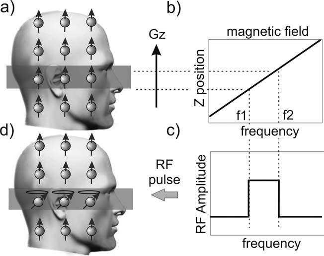
With these ideas in place the process of acquiring an image by playing out a pulse sequence can be described. Firstly, a gradient in the Z-direction, GZ, is applied. Next, an RF sync pulse is transmitted during application of Gz whose bandwidth selects out a rectangular slab of spins along the longitudinal direction and tips them into the transverse plane (Figure 1). Following this, a phase encode gradient is applied to spatially encode the spins along the Y-axis. Next, a frequency encode gradient is applied along the X-axis. During the readout period, the voltage induced in the receiver coils by the rotating transverse magnetization is digitally sampled. A basic pulse sequence is depicted in Figure 2.

Figure 1. A visual depiction of the slice selection process.
The GZ magnetic field gradient induces a linear variation
in frequency as a function of position (b). The desired
slice location and thickness, ΔZ, then corresponds to a
specific frequency bandwidth, ΔF (a, c). By playing out
an RF pulse with the same bandwidth only those spins in
the desired slice are tipped into the transverse plane (d).
Figure 2. A simple MRI pulse sequence. Slice selection
in GZ is applied first along with the RF pulse. Following
this the phase encode gradient along the Y-axis is turned
on, then the GX (or readout) gradient is turned on.
Samples are acquired during the time the readout
gradient is active.
The entire signal acquisition process can be described by the signal equation:
1
where
2
3
The full derivation of (1) can be found in. The key observation is that the exponential term matches that of the two-dimensional Fourier transform. That is, s(t) is the Fourier transform of the magnetization distribution, m. If m lies in image space and is described by spatial location variables <x, y>, then its Fourier transform, M(kx, ky) lies in k-space and <kx, ky> represent spatial frequency. This form reveals that the position in k-space is dictated by the time-integral of the gradients applied. Thus the gradients can be thought of as tracing out a trajectory through k-space. In this case, the Gx (or readout) gradient sweeps from left to right across k-space, and each successive Gy gradient (or phase encode) “blips” the trajectory up another line. As samples of s(t) are acquired over time, k-space is filled in by placing each sample into its appropriate location as given by (2) & (3). An image is then recovered by simple application of the 2D inverse Fourier transform. Most MRI data is acquired using a Cartesian sampling trajectory. That is, k-space is traversed in a raster scan and samples are acquired at regular intervals, <Δkx, Δky>. Samples are acquired along the readout direction with a temporal spacing of Δt, or, a sampling rate of Fs = 1/Δt. The total distance travelled in each direction is given by kx,max = NxΔkx and ky,max = NyΔky, where Nx, Ny are the number of samples acquired in each direction. The reconstructed image then possesses a field of view FOVx = 1/Δkx and FOVy=1/Δky. The distance travelled in k-space gives the resolution: Δx = 1/2kx,max, Δy=1/2ky,max. The scan time for a single frequency encode is the repetition time, given by TR = NxΔt; and therefore for the total image, Timg = TR*Ny. K-space need not be filled in by only a raster trajectory; in principle any arbitrary traversal may be used.
Lastly the source of contrast in an MR image will be described. Immediately following the application of the RF pulse all spins precess at the same frequency and in-phase. However inhomogeneity in the local magnetic field as seen by each spin will cause them to precess at different frequencies. This results in a loss of phase coherence and causes the transverse magnetization to decay over time. Broadly speaking there are two sources of field inhomogeneity. Random interactions of the protons in the form of dipole (magnetic) interactions, thermal rotation, and displacement occur at the microscopic level. Collectively these are referred to as T2 effects and are tissue-dependent.
A second source arises from macroscopic spatial variations that occur in the main field due to imperfect magnet construction, imperfect shimming, and changes in susceptibility at tissue boundaries. These effects are static (or slowly varying) in time and are known collectively as T2′ effects:
4
ΔB is the variation in the field arising from the aforementioned sources. As these effects are external, larger voxels may encompass larger regions of variability, and therefore exhibit greater apparent dephasing. The contribution of both of these effects is known as the apparent T2, or T2* and is shorter than either effect:
5
The overall decay of the transverse magnetization is commonly described by an exponential equation:
6
Where M0 is the magnitude of the transverse magnetization immediately following the RF excitation. It is noted that this is only an approximation and the actual decay function is the Fourier transform of the frequency distribution of spins within the voxel. At the same time, the longitudinal magnetization slowly returns to its original equilibrium value (M0) as excited protons lose energy into the surrounding tissues and realign with the main field. This is known as T1 recovery and is also characterized by an exponential function:
7
Different tissues possess different T1 and T2 (and T2*) values. By adjusting the echo time (TE) and repetition time (TR) of a scan, the resulting image can be weighted towards T1 or T2 contrast. Table 1 shows the effects of different TR and TE values on two tissues with different T1 and T2 values.
Table 1. The left side lists two tissue types and their T1 and T2 values respectively. On the right is a qualitative
description of the resulting image contrast for the indicated tissues.