Optical coherence tomography (OCT)
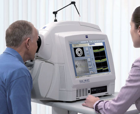
As a high speed, high resolution cross-sectional imaging modality, OCT has been applied in many different areas and is most successful in ophthalmology. OCT is based on a low coherence interferometry, which provides axial resolution through differentiating photons’ optical path length, instead of through the confinement of energy by tightly focusing the optical field, which is also known as confocal gating. Assume the interferometer shown as Figure 2 is illuminated with a broadband light source which has a short coherence length. When a biological sample is imaged, the mirror in Arm 2 is replaced with a sample which reflects light at different depths with different reflectivity. OCT profiles the longitudinal reflectivity at different depth through coherence gate. Corresponding to a reference optical path length determined by the position of Ml, signal photons with the same optical path length as reference light (with uncertainty equals the coherence length of light source) will contribute to the interference signal. Scanning Ml so that the reference optical path length takes different values, the OCT system can detect signal coming from various depths of the sample and therefore obtain a complete longitudinal profile We show the axial point spread function (PSF) corresponding to coherence gating and confocal gating in Figure 2. The blue curve corresponds to the confocal gating of an objective with NA=0.1. The red curve corresponds to the coherence gating of a broadband light source with 20nm FWHM bandwidth. Seen from Figure 2, OCT can achieve a high axial resolution without tightly focusing the probe beam
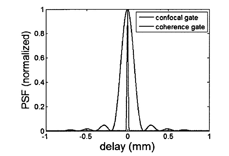
Figure 2 Axial point spread of confocal gating (blue) and coherence gating (red)
In OCT, ID scan (A-scan) is obtained by scanning the optical path length of the reference arm with the probe beam incident into the sample at the same point. Higher dimensional, i.e., 2D or 3D images are obtained by scanning the probe beam in a predefined manner. Shown in Figure3 , ID scan (B-scan)leads to 2D image and 2D scan (C-scan) leads to 3D image.
