Kalman Filter
A Kalman filter is an optimal recursive data processing algorithm. One of the aspect of this optimality is that the Kalman filter incorporates all the information that can be provided to it. It processes all available measurements, regardless of their precision, to estimate the current value of the variables of interest, with use of knowledge of the system and measurement device dynamics, the statistical description of the system noises, measurement errors and uncertainty in the dynamics models, and any available information about initial conditions of the variables of interest. One of the interesting characteristics of the Kalman filter is that it does not require all previous data to be kept in memory and reprocessed every time a new measurement is taken, making the filter implementation more practical. The filter is actually a data processing algorithm, and therefore it incorporates discrete-time measurement samples rather than continuous time inputs. Often the variables of interest, some nite number of quantities to describe the state of the system, cannot be measured directly, and some means of inferring these values from the available data must be generated, thus the need of the filter.
This inference is complicated by the facts that the system is typically driven by inputs other than our own known controls and that the relationships among the various state variables and measured outputs are known only with some degree of uncertainty. Furthermore, any measurement is corrupted to some degree by noise, biases, and device inaccuracies, and so a means of extracting valuable information from a noisy signal must be provided as well. There may also be a number of dierent measuring devices, each with its own particular dynamics and error characteristics, that provide some information about a particular variable, and it would be desirable to combine their outputs in a systematic and optimal manner. A Kalman filter combines all available measurement data, plus prior knowledge about the system and measuring devices, to produce an estimate of the desired variables in such a manner that the error is minimized statistically. In other words, if we were to run a number of candidate filters many times for some application, then the average results of the Kalman filter would be better than the average results of any other
Discrete Kalman Filter
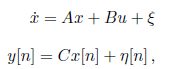
This section is based on the work of. There are several dierent forms of the Kalman filter, but the form particularly useful for Small UAS applications is the continuouspropagation, discrete-measurement Kalman filter. Let’s assume that the linear system dynamics are given by
36
where y[n] = y(![]() ) is the
) is the  sample of y, x[n] = x(
![]() ) is the sample of x,
) is the sample of x, ![]() is the measurement noise at time
is the measurement noise at time ![]() ,
, ![]() is a zero-mean Gaussian random process with covariance Q, and
is a zero-mean Gaussian random process with covariance Q, and ![]() [n] is a zero-mean Gaussian random variable with covariance R. The random process
[n] is a zero-mean Gaussian random variable with covariance R. The random process ![]() is called the process noise and represents modeling error and disturbances on the system.
is called the process noise and represents modeling error and disturbances on the system.
The random variable ![]() is called the measurement noise and represents noise on the sensors. The covariance R can usually be estimated from sensor calibration, but the covariance Q is generally unknown and therefore becomes a system parameter that can be tuned to improve the performance of the observer. Note that the sample rate does not need to be xed.
is called the measurement noise and represents noise on the sensors. The covariance R can usually be estimated from sensor calibration, but the covariance Q is generally unknown and therefore becomes a system parameter that can be tuned to improve the performance of the observer. Note that the sample rate does not need to be xed.
The continuous-discrete Kalman filter has the form
37,38
where L is the Kalman gain. Dene the estimation error as x = x – x. The covariance of the estimation error at time t is given by
39
Note that P(t) is symmetric and positive semi-denite, therefore, its eigenvalues are real and non-negative. Also, small eigenvalues of P(t) imply small variance, which implies low average estimation error. Therefore, we would like to choose L(t) to minimize the eigenvalues of P(t). Recall that
where tr(P) is the trace of P, and are the eigenvalues of P. Therefore, minimizing tr(P) minimizes the estimation error covariance. The Kalman filter is derived by nding L to minimize tr(P). The equations of the Kalman filter can be categorized into two groups: time update equations and measurement update equations. The rst is responsible for projecting forward in time the current state and error covariance estimates to obtain a priori estimate for the next time step. The measurement update equations are responsible for incorporating a new measurement into the a priori estimate to obtain an improved a posteriori estimate.
Time Update Equations
Differentiating x we get
Solving the differential equation with initial condition ![]() we obtain
we obtain
Computing the evolution of P, the error covariance we get
where the 1/2 is because we only use half of the area inside the delta function. Therefore,
since Q is symmetric we have that P evolves between measurements as
Measurement Update Equations
When a measurement is received, we have that
On the other hand we have that
40
To continue our derivation, the following matrix relationship is required:
Our goal is to minimize tr(![]() ) by choosing L. A required condition is that
) by choosing L. A required condition is that
If we substitute into (40) we get
Summarizing the Kalman filter we have two sets of equations. The time update equations, which propagate the state estimates
41,42
where x is the estimate of the state, and P is the symmetric covariance matrix of the estimation error. The second set of equations, the measurement update equations, are used when a measurement is received from the sensor, which updates the state estimates and error covariance with the following equations
43,44,45
where ![]() is called the Kalman gain for the sensor
is called the Kalman gain for the sensor
Extended Kalman Filter
This section is based on the work of. In the previous section we assumed that the system propagation model and measurement model are linear. However, for many applications, including the one used in this thesis, the system propagation model and the measurement model are nonlinear. Therefore the model in (36) becomes
46,47
This case is called the extended Kalman filter. For the EKF, the state propagation and update equations use the nonlinear model, but the propagation and update of the error covariance use the Jacobian of f for A, and the Jacobian of h for C.
Pseudo-code for the continuous discrete extended Kalman filter is given below
Initialize: x = ![]() .
.
Pick an output sample rate that is less than the sample rates of the sensors.
At each sample time :
for i = 1 to N do [Time Update Equation]
Delayed Extended Kalman Filter
In real world applications, measurements usually have processing and communication delays which cannot be ignored. These delays can have big variations, consequently some measurements can arrive in an out of sequence fashion, which worsen the estimations if not handled properly.
In this section we show a modication of the extended Kalman filter, which enables it to handle delayed measurements and the OOSM problem. This filter works by introducing the measurement in the estimation as soon as they arrive, but using it to estimate the states at the time that the measurement was made. After that, this estimation is propagated forward in time. If another measurement more recent is available, then it is incorporated into the estimation and the states are propagated again in time. This is done until the filter is on the current time. Therefore, opposed to how the filter works , this filter can run in real time. For this, we need to store the state estimations, the error covariance ma trices and the delayed measurements for as many time steps as the maximum probable delay.
Pseudo-code for the continuous discrete delayed extended Kalman filter is given below