Instructor Pilot Interviews

Studying pilot fatigue through flight dynamics has never been attempted before which manifests one question, where to start?
For a study on pilot fatigue in which none of the researchers had any flying experience, it made sense to begin by getting the opinions of expert pilots. Lear Siegler Services Incorporated has been honored to be the U.S. Army’s rotary wing flight trainer
since 1989. They have trained over 20,000 Army, Air Force, and Allied students to meet their world-wide commitments as military rotary wing pilots. They serve at the U.S. Army Aviation Warfighting Center, Fort Rucker, Alabama, which is the largest
helicopter flight training school in the world17. Most of the instructors at this school have more than 6000 hours of flight experience, and since the U.S. government trusts them to train their military pilots, their answers to specifically designed questions should add substantial backing to any piloting research.
The purpose of pilot interviews was to gain firsthand knowledge in dealing with fatigue. Every pilot interviewed had extensive experience with both rotary and fixed wing aircraft. Even though experimental data used for this research was gained from a
fixed wing flight simulator, pilot fatigue related to flying rotary and fixed wing aircraft were equally considered at this point in the research process. Interview questions and responses can be found in Appendix C.Among those interviewed was Program Manager of Lear Siegler at Fort Rucker retired Army Colonel Charles L. Gant. Colonel Gant is a former Master Army Aviator
and instructor pilot17. Colonel Gant has roughly 6000 rotary wing flight hours and upwards of 1800 fixed wing flight hours and has flown over 25 different types of aircraft.
When asked if he perceived the aircraft to respond differently when tired Colonel Gant stated that his “fine touch control skills diminished.” This loss, or reduced ability to carry out otherwise normal ‘rested’ piloting functions is exactly what this research will prove is detectable. Along with skills diminishing, Ed Gruetzenmacher, another instructor pilot at Fort Rucker who has over 7000 total flight hours spread over roughly 25 different aircraft,added that when fatigued his “response time was slower.” Slower reaction time is a symptom of fatigue that can lead to accidents, especially in landing approaches when the
pilot must be fully alert.
In response to a question asking about having to work the controls more when tired to achieve the same aircraft performance Mr. Gruetzenmacher stated that when he was “not as alert, the airplane seemed to wander” off course. This answer again supports the main hypothesis and assumptions that this research effort is based on. The aircraft wandering off course should show up on elevation sensors as well as adding detectable variance of other state variables such as sideslip angle and roll attitude angle.
In addition to obtaining information about flight conditions when fatigued, other questions were asked in order to learn about other potential sources of fatigue for future studies. One question that was asked of all pilots from Fort Rucker was, “What
environmental conditions such as the sun, wind, rain, clouds, night flight, etc. hasten your fatigue?” Every pilot agreed that some if not all of these factors took a toll on them during flight. Dale Kiel, a former army pilot with over 14,000 flight hours, commented that “flying in the clouds with turbulence” put the most strain on his ability to control his aircraft efficiently. Though flying through clouds was not included in this study,turbulence was definitely part of the flight scenario that every test pilot used for this study had to deal with. Mr. Kiel also added to Colonel Gant’s comment concerning reduced ability to control the aircraft. Mr. Kiel said that when flying in a ‘tired’ condition he noticed that his response time deteriorated. Future studies using the delay
variable found in the human operator models mentioned in the background would be supported by the testimonies of Mr. Kiel and Colonel Gant.
Interviewing the flight instructors from Fort Rucker provided significant support confirming both the utility of this research effort and the assumptions it was based on.
The interviews validated that the aircraft should show signs of dynamic change in the presence of a fatigued pilot. Words such as the ‘loss of fine touch skills’ had the conclusion that the pilot would have to provide more compensation to keep the aircraft on course. Remarks such as this also provided a positive outlook in finding that there should indeed be an increase in standard deviation and mean of the tracking errors of the state and control variables, which is what the detection schemes would be monitoring in order to classify either a ‘rested’ or ‘tired’ pilot condition. The statements mentioning boredom
causing fatigue on long flights led to the belief that fatigue detection would be very successful for the steady level flights. In addition to solidifying hypotheses made in the beginning stages of research, the interviews gave vital support for other areas of research related to fatigue detection discussed in the background section such as the possible
fatigue detecting variables within the mathematical models.

 

Flight Simulator

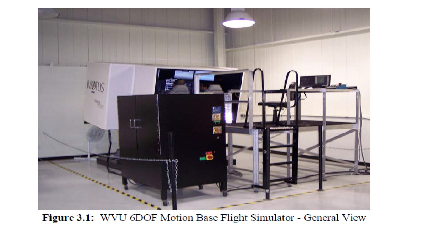
The WVU College of Engineering and Mineral Resources’ Mechanical and Aerospace Department 6 degrees-of-freedom flight simulator was used for this research effort. The Motus 600 Flight Simulator18 shown in Figure 3.1, manufactured by Fidelity
Flight Simulation offers a realistic flight environment allowing “true” motion cues flight simulation capabilities using electric actuators. A 140° four-monitor, wrap-a-round external visual display provides high quality visual cues.
The Laminar Research X-Plane19 flight simulation software is used to drive the simulator system. X-plane19 is a commercial comprehensive aircraft simulation package featuring high capabilities and flexibility in selecting the simulation scenario. The
software saves the data during the simulation so that selected parameters can be analyzed later. Also, the software has the ability to simulate still air conditions as well as varying levels of turbulence. The cockpit accommodates dual controls and instrument clusters. Visual information in the cockpit is provided by a total of 6 LCD visual displays which can be seen in Figure 3.2. Two displays host the instrument clusters and the other four provide external visual cues. Flight scenario set-ups/changes and monitoring the simulation are preformed from the operating station located to the right of the cabin in
Figure 3.1.

 

Test Pilot Acquisition

The next step in the experimental phase was finding pilots for the study. Five WVU Aerospace Engineering students with flying experience volunteered for the project. Among the five pilots, three of them were considered experimental and the other two
were used for validation purposes only. The data collected from the experimental pilots was thoroughly examined and used for analysis. The validation data from the other two pilots was only used at the end of the project to verify the designed detection schemes as results will show, the scheme shows definite implementation potential.

Test Pilot Classification ~ Rested/Tired

The CHS Alertness Model6 from Chapter  Figure  was utilized for the purpose of ensuring either a ‘rested’ or ‘tired’ pilot condition. Based on the model, the students were given specific instructions on when to wake up depending on which test
they were flying that particular day. The times of the tests were scheduled based on actual waking time and time since last sleep to guarantee that the pilots were verified as ‘rested’ or ‘tired’ according to the Alertness Model6.
Each pilot was given a post flight questionnaire, which consisted of ten questions that were designed to gain additional information regarding the pilots’ condition and performance (see Appendix B). Questions one and two let the researchers know when each pilot woke up and roughly how long each one slept. Questions two and three centered on the quality of sleep and how rested the pilot felt upon waking. Questions five and six gained information regarding any substances that could have altered the pilots flying ability such as any medications taken as well as roughly how much caffeine was consumed prior to simulation. Questions seven through ten were designed to allow each pilot to comment on their performance.

 

Flight Scenario

3.5 Flight Scenario
A flight scenario was developed for the simulation that incorporated different types of maneuvers. Each pilot flew the scenario while ‘rested’ and then again when ‘tired’. The test pilots were given a chance to study the scenario and take two practice
flights before any data collection took place. The following was the complete flight scenario flown by each pilot. The average duration of each simulation was approximately 40 minutes.
1. Take-off.
2. Climb up to 1000 ft AGL at 110 knots.
3. Steady climb up to 3700 ft AGL at 140 knots.
4. Maintain steady state level symmetrical uniform flight for 1 minute at 3700 ft and
140 knots.
5. Perform a coordinated turn, full circle to the left, at 45° and 140 knots.
6. Maintain steady state level symmetrical uniform flight for 30 seconds.
7. Accelerate up to 160 knots in 3 minutes.
8. Decelerate back to 140 knots in 3 minutes.
9. Maintain steady state level symmetrical uniform flight for 30 seconds.
10. Decelerate to 90 knots (use landing gear and flaps).
11. Perform left coordinated turn, full circle at 5°.

12. Maintain steady state level symmetrical uniform flight at 90 knots with maximum
turbulence for 4 minutes.
13. Perform a coordinated turn to the left with turbulence at 5° for a full circle.
14. Perform a coordinated turn to the right with turbulence at 5° for a half circle.
15. No turbulence, accelerate back to 140 knots.
16. Maintain steady state level symmetrical uniform flight for 30 seconds at 140
knots.
17. Perform a pitch attitude doublet (+10° and –5°) while maintaining altitude,
velocity, and heading.
18. Maintain steady state level symmetrical uniform flight for 30 seconds at 140
knots.
19. Perform a roll attitude doublet (±60°) while maintaining altitude, velocity, and
heading.
20. Maintain steady state level symmetrical uniform flight at 140 knots with
maximum turbulence for 6 minutes.
21. Cancel turbulence, prepare for landing.
22. Follow the same standard procedure to land.
There were 10 of the total 22 steps in the flight scenario identified as maneuvers
for this investigation. Each maneuver was given its own number that will be referenced
from here on. However the following table identifies the step number within the scenario
and defines the corresponding maneuver and new maneuver number.

Table : List of Maneuvers Chosen from Flight Scenario for Fatigue Study

 

During a steady level flight the pilot was to keep the aircraft level, on heading,at the specified speed and altitude. The turns required the pilot toeither a full or half circle turn while keeping a preset bank angle, velocity, and constant throughout the maneuver. For the roll doublet, starting at steady level , the pilot first rolled the aircraft 60° to the left, then back through zero to 60° to the , and ended the maneuver by returning to steady level flight. For the pitch doublet, at steady level flight, the pilot pulled the nose of the aircraft up 10°, then back zero down to -5°, and ended by returning to steady level flight.

Data Processing

The time histories of each variable were recorded in matrix form in a .out file.Each column within the matrix corresponded to a different parameter. Due to the 40 minute test duration the size of the file from the simulation software was extremely large.
This file could be opened in Microsoft Word® but numerous undesirable format characters were spread throughout the file and had to be eliminated before the data could be transferred to Matlab® and used for analysis. Because the raw data files were so large, they had to be divided into 10-15 smaller files in order to remove all of these characters in a timely fashion. Once these unwanted characters were removed, the data from the 10-15 separate files was saved as a Matlab data file. With the data formatted, the next step was to pick out the individual maneuvers for each pilot’s simulation.

Maneuver Identification

In order to determine the specific maneuver intervals Matlab was used to plot five state variables for the entire duration of the simulation. Only example plots will be included as the process was the same for each pilot and because the graphs looked so
much alike for each specific maneuver. The variables plotted were velocity, roll, pitch, and yaw attitude angles  and angle of attack  Figure  is an example of how the entire simulation would appear.

Using the flight scenario outline in conjunction with the outputs from the selected variables each maneuver can be identified. The first maneuvers identified were the coordinated turns as they were the easiest to detect using roll angle and yaw angle
For example, the way to identify maneuver number five, a coordinated turn with a 45° banking angle, is to look for when yaw angle goes through a complete 360° cycle and when roll angle goes to negative 45°. This happens at roughly 400 seconds into the simulation. The other turns were identified using this same procedure. When identified and isolated, the maneuver will appear as displayed in Figure

In order to use the data for analysis, yaw angle had to undergo additional to get rid of the jump from zero to 360 degrees. The jump is a consequence of how the flight simulator measures the yaw angle value internally. It measures values of
yaw attitude angle from 0 to 360 degrees only. A simple ‘for’ loop was used within Matlab to shift the second half of the data downward so that yaw angle ranged from roughly 180° to -180°, which made the analysis much easier. At no time during the
filtering was the integrity of the raw data compromised. Figure 3.5 is characteristic of what the usable data for the coordinated turn will look like.

The next maneuvers identified were the doublets. A doublet is simply defined as back and forth rocking of the aircraft. A roll doublet means that while maintaining heading and speed the plane will roll to one side and then other ending up back at level flight. A pitch doublet means the aircraft will go nose up, then nose down and again return back to level flight. In these maneuvers the pitch and roll attitude angles were used for identification. For the pitch doublet, pitch angle goes from zero to +10° to -5° and then back to zero. The roll doublet called for roll angle to go from zero to +/-60 to – /+60 and then back to zero. Unlike the pitch doublet, for the roll doublet the pilot was not ordered to go either left or right first as it did not matter for this study. However, as the ‘rested’ case was considered the reference, pilots were ordered to repeat the same first direction during their ‘tired’ simulation. Figures 3.6 and 3.7 show both the pitch and roll attitude doublets respectively.

The next type of maneuver to identify was steady level flights. During these maneuvers the pilot was instructed to keep velocity, altitude, heading, etc. constant. Most steady flights were used to break up the sequence of other maneuvers. Therefore, once the other maneuvers were identified, the steady level flights became the data occurring between most maneuvers. For example, each pilot was to perform the pitch doublet then go into a steady level flight for 30 seconds before continuing with the roll doublet. Knowing that the steady level flight occurred between these two maneuvers and having  already located the doublets, the steady level flight condition could be properly identified. A characteristic steady level flight condition can be observed in Figure 3.8. There were two other steady level flight conditions, but they were executed during simulated turbulence.
The simulator can produce flight conditions that mimic realistic interferences that a pilot flying an actual aircraft could encounter, one of which is turbulence. There is a mechanism within the X-Plane19 software that allows the user to set the amount of turbulence the pilot will encounter. For the purposes of this study maximum turbulence was selected for all maneuvers in hopes that the more severe the turbulence the easier it would be to see greater variances between the ‘rested’ and ‘tired’ state variables. Turbulence was simulated for both coordinated turns and steady level flights. The methods for finding these two types of maneuvers without turbulence were used again when identifying them in presence of turbulence. Looking back on Figure 3.3 there are noticeable areas of data that appear chaotic as compared to rest of the data. These chaotic areas were due to the introduction of turbulence. Figures 3.9 and 3.10 represent characteristic plots of both a steady level flight and a coordinated turn in turbulence.
The maneuver identification process was the last step leading up to analyzing each state and control variable for their fatigue detecting capabilities. As stated, the plots and specific maneuvers discussed in this section are examples of the corresponding maneuvers.

Analysis Tools

This research effort required constant use of Matlab programs to load data sets for each pilot and maneuver for analysis. Graphical User Interfaces (GUIs) were created to make this process quick and consistent. Figure 3.11 displays the first GUI created. The GUI allowed the user to select maneuver type, pilot, and which metrics were to be calculated second GUI, in Figure was created for the composite variable analysis and implementation of the detection schemes.