In order to proceed with analysis of the data it is very important to have a data mining process.
There are various data mining methodologies; these methodologies attempt to shape the way a data analyst approaches the steps to perform the data mining tasks. The two major methodologies that are most used are SEMMA and CRISP- DM. SEMMA, which stands for Sample, Explore, Modify, Model, Assess, has been developed by SAS Institute. On the other hand, Cross Industry Standard Process for Data Mining (CRISP- DM) was developed by software vendors and industry users of data mining. For this study, the data mining process that is being used is a Cross Industry Standard Process for Data Mining (CRISP- DM) approach. This approach consists of six phases.
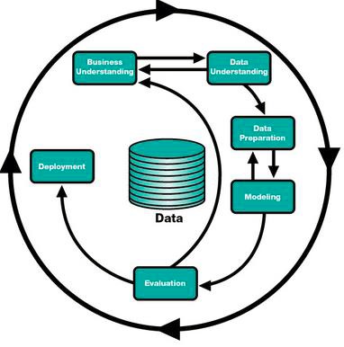
Business Understanding
This is the initial phase of the process where the business question or the question of interest is discovered. In this study the research question is, what factors contribute to survivability of an ovarian cancer patient? Also, are there any patterns a patient needs to pay attention to in terms of getting early cancer treatment?
Data Understanding
The given data is examined for the appropriate data type and knowledge is acquired about the various tables and variables available in the dataset.
Data Preparation
To prepare the data for analysis the following sub steps were used:
a) Data Access
The study uses the data from the Center for Health System Innovation (CHSI) provided by Cerner Health Facts. The Cerner Health Facts dataset is the largest relational database on healthcare. This database is a comprehensive source of de-identified, real-world, HIPAA-compliant data.
The database consists of more than 50 million unique patients, more than 2.4 billion laboratory results, more than 84 million acute admissions, emergency and ambulatory visits, more than 14 years of detailed pharmacy, laboratory, billing and registration data and more than 295 million orders for nearly 4,500 drugs by name and brand.
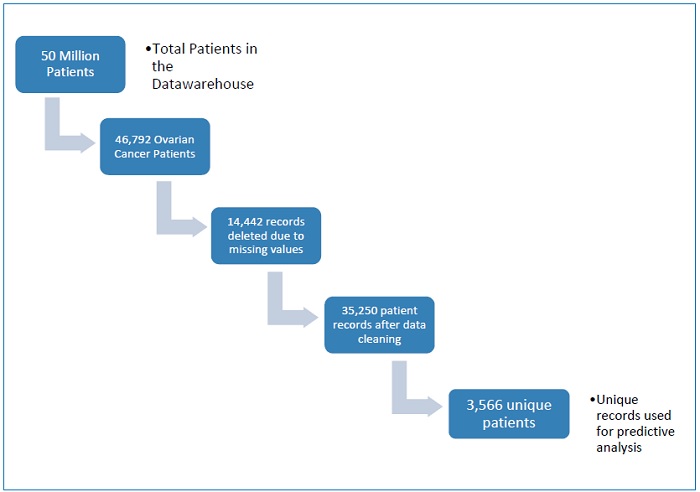
The data for ovarian cancer patients is extracted using the SQL Server Management Studio 2012. SQL is a standard language for accessing and manipulating databases. Since, Cerner Health Facts® is a Relational Database Management System the basis to use it is SQL. The flow chart Fig.2 shows the steps followed in the extraction process. There were more than 50 million unique patients, more than 14 years of detailed pharmacy, laboratory, billing and registration data and more than 295 million orders of drugs by name and brand. These were filtered and 46,792 ovarian cancer patients were considered. Later, these were brought down to 32,350 patients’ records which had the desired information related to survivability of these patients. Out of these 3,566 were unique patients, are useful for analysis of this study. These records were obtained using SQL and SAS software when required. Clauses, expressions, statements etc. were widely used in the data extraction process from SQL server.

Fig2 Process flow of data extraction
b) Data Consolidation
The data was acquired in a text (.txt) file and was then brought into SAS enterprise Guide (6.1) this text file was converted into a .sas7data file. There were no major issues while consolidating the data.
c) Data Cleaning
The raw text file consisted of 80 variables. The dataset had more than one Encounter_ID,
Hospital_ID, Patient_ID, Dischg_disp_ID, Procedure_ID etc. so the duplicate columns were
deleted and only one of each column was kept. Other variables like age_in_months, age_in_weeks, and age_in_days etc. were dropped as all the records had all “0” values, this is observed using histograms and analyzing the mean, minimum and maximum. Since the data set also consisted of the variable age_in_years the other age related variables didn’t serve any purpose. Further, initial data exploration was conducted on each variable through descriptive statistics. For interval variables, the mean, minimum, maximum, and missing values were studied.
Histograms were used to analyze the distribution of these interval variables. To check if there were any outliers box and whisker plots were used for interval variables. Very few records consisted of missing values. Once all the duplicate columns were removed and outliers were analyzed another step was essential to use the data for analysis. Since, each record in the data set captures the encounters of the patients visit to the facility. Which implies there can be multiple encounters for a particular patient.
As this study focuses on the survivability it was important to have single encounters of these patients. To do so the records were aggregated for the same person using the patient_sk variable that is unique for a particular patient. There are other data challenges that needs to be accounted for like the curse of dimensionality. The curse of dimensionality, an expression coined by mathematician Richard Bellman, refers to the exponential increase in data required to densely populate space as the dimension increases. In case of a large number of inputs the curse of dimensionality doesn’t fit the model so well. In this study, this issue was handled by reducing the total number of inputs from 80 to 45. The problem of redundancy occurs when the input doesn’t give any new information that has not already been explained. The dataset did have redundant variables for example: dischg_disp_id and dischg_disp_code these two variables explain the same information about the patients’ discharge status similarly other variables were discarded based on redundancy. After cleaning of data the variable list was brought down to 47.
Modeling
Data mining is also about model generation. This step involves using actual modeling techniques that can be used to address the research question. Data mining models can be generated for three types of tasks like: descriptive profiling, directed profiling and prediction. The descriptive models or descriptive profiling gives insight into what the data does. Outputs of these models and hypothesis testing generate graphs, charts and summary statistics of the data. Direct profiling is when the target and the inputs for the models are from the same time frame. Prediction is finding patterns in the data from one period that are capable of explaining outcomes in a later period. This study focuses on both Predictive modeling and descriptive profiling.
Evaluation
The task in this step is to evaluate the generated model and go back and forth to reach the desired outcome for the research question.
Deployment
The last step is report generation and summary of the project.