Artificial Neural Network Design and Implementation

Neural network structure and model

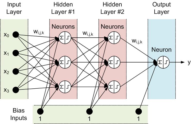
In this work, a multi-layer feed-forward neural network (FFNN) is proposed as shown in Figures 3.1 and 3.2. The Levenberg-Marquardt Back Propagation (LMBP) method is selected for training the ANN network to increase convergence speed, and to avoid long training times. The LMBP algorithm is based on numerical optimization techniques and is a generalized form of the Least Mean Square (LMS) algorithm.Backpropagation (BP) is an approximate steepest descent algorithm, in which the performance index is mean square error. The difference between the LMS algorithm and backpropagation is in the way in which the derivatives are calculated. In multi-layer networks with nonlinear transfer functions, the relationship between the network weights and the error is more complex than single-layer networks. In this case, for calculating the derivatives, the chain rule is used. Backpropagation method is usually used in supervised learning and the input and desirable outputs are provided for the network and then the weight matrix of the network is updated and adjusted to minimize the error function by calculating the gradient of error function

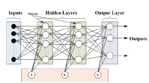
Figure 3.1 Feedforward Neural Network schematic

Figure 3.2 Feedforward Neural Network: mathematical description

First, we start from simple backpropagation algorithm; then, we discuss the LMBP algorithm. For a multi-layer network, the output of one layer becomes the input to the next layer with the following equation :

where ? is the number of layers in the network, ? is the weight matrix, ? is the bias vector, ? is the activation function to calculate the output values of each layer, $a ^{m}$ is the input vector, and $a ^{m+1}$ is the corresponding output (input for the next layer). The algorithm should adjust the network parameters to minimize the mean square
error :

Where ? is the vector of network weights and biases. Considering a network with multiple outputs, the error function can be generalized to :

where ? is the error function, and ? is the desirable target vector.
The steepest descent algorithm for approximating mean square error is :

where ? is the learning rate and ? is the iteration steps. In multi-layer networks the error is not an explicit function of the weights in the hidden layers, therefore these derivatives are calculated with complexity. Hence, the chain rule is used to calculate the derivatives as follows :

where $s^{m}_i\equiv \delta_F/\delta_n m^{i}$ is defined as the sensitivity of ? to changes in the ??ℎelement of the net input at layer ?.

Then, we car rewrite (3.4) and (3.5) as:

where

The next step is to calculate sensitivity matrix. This requires a recurrence relationship in which the sensitivity at layer ? is calculated from the sensitivity at layer ? + 1. This is the reason why this method is called backpropagation. To derive the recurrence relationship for sensitivities, the following Jacobian matrix is used :

Next, each element of the Jacobian matrix is obtained using :

Therefore the Jacobian matrix can be written as :

Now the recurrence relation for the sensitivity by using the chain rule in matrix form is obtained using :

The sensitivities are propagated backward through the network from the last layer to the first layer :

In last step of the back propagation algorithm, we need to calculate the $S^{M}$ for the recurrence relation in (3.22). This is obtained at the final layer :

Levenberg-Marquardt Backpropagation Algorithm

The Levenberg-Marquardt backpropagation algorithm is a variation of Newton’s method that is designed for minimizing functions that are sums of squares of other nonlinear functions. This algorithm is very well suited for training neural networks where the performance index is the mean squared error. Starting from Newton’s method for optimizing a performance index ?(?)

Considering ?(?) as a sum of squares function

Then the $j^{th}$ element of the gradient is obtained

The gradient can be written in matrix form as :

where ? is the Jacobian matrix and obtained as follows :

After this step, the Hessian matrix is obtained as follows :

The Hessian matrix can be written in matrix form as :

By assuming ?(?) to be small, the Hessian matrix can be approximated as :

Then the Gauss-Newton method is obtained as follows:

The advantage of Gauss-Newton over the standard Newton’s method is that it does not require computation of second derivatives. The problem with the Gauss-Newton method is that the matrix ? = ?? ? may not be invertible. This problem is solved by using the following modification:

In the above modification, ? can be invertible by increasing ? until (?? + ?) > 0 and ? becomes positive definite. This modification will result in Levenberg-Marquardt algorithm:

In the Levenberg-Marquardt algorithm, by increasing $\mu_k$ it approaches the steepest descent algorithm with small learning rate. However, by decreasing $\mu_k$ to zero, the algorithm becomes Gauss-Newton.
The Levenberg-Marquardt algorithm is applied to the multi-layer network training problem as follows. The proposed LMBP training algorithm can be derived briefly as follows

In a multi-layer network, layer output can be calculated as :

where ? is the number of layers in the network, $w^{h}_i_j$
ℎ is the weight value with respect to the $j^{th}$ elements of input vector and the $i^{th}$ neuron of layer ℎ, ? is the size of input vector, $b_i ^{h}$ is
the ith element of bias vector for layer ℎ, ??? is the activation function to calculate the output values of each layer, $a_j ^{h-1}$ is the input vector, and $o ^{h}_i$ is the corresponding output for layer ℎ.The gradient method is used with the following computation to minimize the mean square error:

where ? is learning rate, ? is the iteration steps, ? is the error function, ? is the vector of network weights and biases, ? is the input vector, and ? is the desirable target vector. According to the chain rule and the derivative of the error function with respect to the weights and biases, (2) and (3) can be rewritten as:

using Δ??,? ℎ and Δ?? ℎ to minimize the error function.

Then the Jacobian matrix is calculated using :

The change of error in each step of iteration is calculated by:

where ? is defined as damping factor. Then the sum of squared errors is calculated using

The measured error in each step of iteration has to be smaller than its previous value until it reaches a specific desirable error deviation Δ(?) for stopping criterion.

ANN training and implementation

Training process is the most important step in design of a neural network. For solving cascading failure problem based on the generators’ power adjustment using the ANN intelligent method, a three-layer feed-forward neural network including two hidden layers and one output layer is considered. In the supervised ANN, a group of input and target samples are required for training process. The input and target patterns are provided such that inputs are defined as limited set of transmission lines tripping combinations due to the line congestion in a binary coding combination of {0, 1}. The corresponding targets are defined as a set of actions (±Δ $P_G_i$ , ? = 1,2,3) for power adjustment in the system through frequency control of the generators. The number of neurons in the input layer is determined by the number of transmission lines. The number of neurons in the output layer is determined by the number of the generators since the output of the trained network is the output power adjustment action (±Δ $P_G_i$ ) from the generators. The term Δ $P_G_i$ is defined as a change in the output power of the $i^{th}$ generator. This power adjustment action is considered as a signal with discrete value and discretized into {-1, 0, 1} for each generator.
The {-1} corresponds to the −Δ $P_G_i$ as a decrease in the output power, {0} indicates no change in the output power, and {+1} corresponds to Δ $P_G_i$ as an increase in the output power. This change in the output power is made by a change in the input frequency through frequency control unit. For the two hidden layers and the output layer, ‘log-sigmoid’ and ‘linear’ transfer functions are used, respectively. These functions are defined in Figs 3.3 and 3.4. The weight and bias networks are initialized and configured for the training process. We choose fixed values to initialize the weight and bias sets for better performance rather than random configuration. In fact, random initialization brings about different weight and bias sets at each training step due to the sensitivity of error function to the weights and biases.

Log-sigmoid function :

Figure 3.3 Log-sigmoid transfer function

Linear function:

Figure 3.4 Linear transfer function

Table 3.1 Proposed ANN training parameters

Then, the weight and bias sets are adjusted during the training process according to (3.44) and (3.45) to minimize the error function. We utilize the MATLAB/SIMULINK to train the proposed algorithm. The parameters of the training process are listed in Table 3.1.Appendix B also shows a part of the real-time ANN program in Visual Studio for integration of the ANN-based control algorithm with LABVIEW program and hardware setup.Training performance of the proposed ANN can be investigated by three indices defined as train, test, and validationas shown in Figure 3.5. The data set is categorized into three groups. The first one is the training set, which is used for the steepest descent calculations and adjusting the weight and bias sets. The second one is the validation set in which the error is measured during the training process. The test subset is not used in training, but is utilized to monitor the test set error during the training process

Figure 3.5 Evaluation of the proposed ANN training process: regression evaluation

Artificial Neural Network Design and Implementation

Neural network structure and model

Levenberg-Marquardt Backpropagation Algorithm

ANN training and implementation

Log-sigmoid function :

Linear function:

Submit a Comment Cancel reply

Cart

Troubleshooting and online tutorials

Product Categories

Product tags