In this section, some tests were designed to compare the capabilities of TIS G1 and TIS G2 in characterizing an inclusion embedded in the soft tissue. The models are developed using spherical targets and PVC tissue phantom with base, depth, and intermediate layers. Figure 2 shows the schematics of PVC tissue phantom. We will perform depth, size, and elasticity tests using different targets and depth layers.
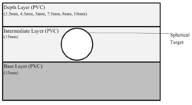
Figure 1: The Schematics of PVC Tissue Phantom
For the depth estimation test, the target is a 15.54mm polyacrylonitrile ball. We record the average minimum normal forces for six different depth layers (3.5mm, 4.5mm, 5mm, 7.5mm, 8mm and 10mm). The 5mm data is used as test data, others are training set data. After we build the models for TIS G1 and G2, we will test the 5mm data and calculate errors. Secondly, we try the size estimation test using 4.5mm depth layer and five different polyacrylonitrile balls (10.71mm, 11.81mm, 13.73mm, 15.54mm and 17.88mm). We will also build the models and compare the errors.
To begin the elasticity accuracy experiments, we need to create target samples. Since it is difficult to determine the true elasticity of objects, we are attempting to measure the relative elasticity. As previously discussed, PDMS has two main mixing components: A, the base agent and B, the curing agent. Increasing B increases the elasticity of the PDMS. Elasticity samples created for testing the accuracy made from different ratios of PDMS (1:20, 1:15, 1:10, 1:5 and 1:1.4). After we have all of our samples created, we can begin testing In the same manner as for size and depth test, we will calculate errors and compare them.
Statistical Analysis Methods
To compare the accuracy of TIS G1 and TIS G2, we will repeat the experiments multiple times to get statistical data and perform statistical analysis. This will compare the performance of these two systems. we will describe the statistical analysis methods that we use in this thesis.
Student’s T-test
Student’s t-test is one of the most commonly used techniques for testing a hypothesis on the basis of a difference between sample means. A two-sample t-test examines whether two samples are different and is commonly used when the variances of two normal distributions are unknown and when an experiment uses a small sample size.

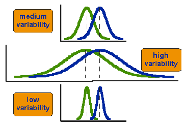
Figure 2: Three Scenarios for Different Distributions (Trochim, 2006)
Figure 2 shows three different scenarios for different distributions. From the three scenarios, we can find that the differences between means are small in the three cases, but these three situations are not same (Trochim, 2006). The first one shows the data in each group has moderate variability. The second one shows the data in each group has large variability. The third example shows the data have small variability. After comparing the distributions in three cases, we could notice that the two group data in third situation appear most different or distinct. For the third case, the two groups’ data overlap so much, so the difference is least striking. We can conclude that when we consider the difference between two groups, we should compare the means with the variability. Therefore, t-test will be used to look up the statistical difference between two groups.
In t-test, we will calculate the t-value, which is a ratio of signal over noise. The signal part is the difference between the two means or averages and the noise part is a measure of the variability or dispersion of the data. The formula of t-value is shown below,
The top part of the formula is easy to find and just uses the mean of second group and subtract the mean of first group. The bottom part is little complex, the standard error of the difference is used to represent the variability of groups. The formula of the standard error of the difference is shown below,
The var1 and var2 are the variances for each group and the and are the numbers of samples in each group. We first divide variance by the number of smaples for each group, add these two values, and then take the square root. After we find out the t-value, we can check the value with a table of significance to see if the ratio is large enough to say that the difference between the groups is statistical significant. To test the significance, we need to set a risk level and it usually to set the alpha level to 0.05 in most research.
To perform t-test, JMP Pro 10.0.2 will be used in our statistical analysis. JMP combines powerful statistics with dynamic graphics, in memory and on the desktop. Its interactive and visual paradigm enables JMP to reveal insights that are impossible to gain from raw tables of numbers or static graphs. We can easily perform t-test from our data using JMP.
Another Possible Statistical Analysis Method
In our size estimation algorithm, we calculate diameter of the target from applying force and pixel numbers of correlative image for each depth layers. In this method, we can use principal component analysis(PCA) to compare the fitting module and differentiate the data in several groups. PCA is a mathematical variable reduction procedure. It converts a larger number of observed variables into a smaller number of variables. Number of original variables is more than or equal to the number of principal components. In this technique, the first principal component has the highest variance; the second principal component has the second highest variance and so on. But each principal component should be orthogonal to the one before that.
PCA helps us to identify pattern in data and emphasize on the similarities and differences of the dataset. When the data had a large number of variables, patterns in the dataset are difficult to be recognized. So we can use it to differentiate our size data for different depth layers. We can use the PCA plot tool in the software Unscrambler for this purpose.