Shortest Electrical Distance (SED) Based Method

One method for moving generators whole is known as the shortest electrical distance (SED) method. The SED method, moves each external generator to a boundary bus via the shortest path in terms of electrical distance. There are many definitions of electrical distance. Here the electrical distance of a path between two buses is the sum of impedances (reactance with dc assumptions) in that path.

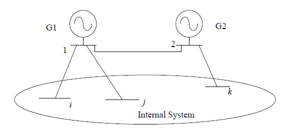
Fig. 1 Example to show electrical distance

As shown in Fig. 1, for generator G1 there are three possible paths to boundary buses: path 1 is from bus 1 to bus i, path 2 is from bus 1 to bus j and path 3 is from bus 1 to bus k via bus 2. The distance of path 1 and path 2 are same as reactance values of the lines connecting the two buses. For path 3, the path distance is the sum of the reactances of the line connecting bus 1 and 2 and the line connecting bus 2 and k. The shortest path can be found using Dijkstra’s algorithm.
The SED method is an optimal method in terms of finding the minimum electrical distance. Its accuracy in terms of approximating the full-model dc OPF results will be studied and discussed in the following.

Optimization Based Generator Placement (OGP) Method

Formulation

The OGP method places external generators on retained buses by solving an optimization problem. The formulation of the problem shares aspects of the dc OPF formulation as it is applied to the reduced model.
Recall that for the dc OPF formulation, the LMP is influenced by two system features:
the marginal energy cost, which is a function of the generation mix, and marginal congestion cost, which is a function of generator location (which may be thought of as a feature characterized by topology and branch parameters.) When producing a reduced equivalent the generation mix is fixed. Given that the topology and branch parameters of a network equivalent are also determined by Ward reduction, the only remaining free variables available to match the marginal congestion cost component of the LMP’s are the placement of generators, placement of the loads, or both, so that congestion in the full and reduced models is maintained.
With the strategy mentioned above, formulation of the generator placement problem can be made by somewhat generalizing the dc OPF formulation applied to the reduced model with binary variables added to specify generator placement. A set of new variables are introduced.

To balance power generation and consumption, the external load should be moved to a retained bus. In the OGP problem, each external load is also moved to one “appropriate” retained bus. Similar to moving generators, a set of binary variables is introduced:

Since the new set of variables are binary, the optimization problem becomes a mixed integer programming (MIP) problem. The objective function can be written as

Two components are included in the objective function. The first component minimizes generation cost which maintains similarity between the OGP solution and the reducedmodel dc OPF solution. The second component minimizes the flow error on the retained congested lines between the full-model dc OPF solution and the OGP solution. In the second component, $P{^f}{_{j,full}}$ , is the line flow (MW) on branch j which is assumed to be a priori knowledge. Since line j is congested, the line flow is actually the same as the limit. As formulated, the OGP benefits from knowledge of the full model dc OPF results or the congestion profile in the full system.
In the second component of (1), the parameter $W_j$ is the weight of line-flow error of the congested line j. It is important to assign an appropriate value to $W_j$ . The effects of different weight assignments will be discussed later in this chapter and a tentative strategywill be proposed.
The constraints of the OGP formulation can be divided into four groups. The first group is the modified reduced-model dc OPF formulation:

2,3,4,5

where $K_I$ and $K_E$ are the sets of internal and external buses respectively and $j_f$ and $j_t$ are
the indices of the from and to end buses.
The second group of the constraints are configured to assign external generators to
retained buses:

6,7,8,9

Constraint sets (6) and (7) impose limits on the external generators. Constraint set (8) ensures that each external generator is moved to one and only one retained bus. A third group of the constraints assigns each external load to a retained bus:

10,11,12

Constraint set (10) guarantees that the load at each external bus is moved to an “appropriate” retained bus. Note that after placing the external generators and loads by the OGP method.

In the objective function, (1), the second component involves calculation of the absolute value of line-flow errors. Calculation of the absolute value can be reformulated into linear expressions. The reformulation involves a set of variables t and also a group of constraints:

13,14

Constraint sets (13) and (14) indicates that $t_j$ is greater or equal to the absolute value of the line flow error. The objective function can be updated as:

As shown in (15), the OGP problem is a minimization problem and the weights are all positive. In the process of solving the problem, $t_j$ will be equal to the absolute value of the flow error. Consequently, the OGP problem formulation includes the objective function (15) and constraints (2)-(14).

Shortest Electrical Distance (SED) Based Method