Q-learning
Even the value iteration algorithm is not the solution to every problem especially where the cost and the transition probability functions are unknown a priori, so the value iteration algorithm can not be used to compute the optimal value function. Instead we need to learn it online, based on experience.
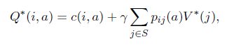
So, we need some model-free RL approach like Q-learning. The main advantage of Q-learning is that it is able to compare the expected utility of the available actions without requiring a model of the environment. The optimal action-value function (Q-function) can be defined as
3
where is defined in (2). In words,
 is the discounted cost achieved by taking action a in state i and following the optimal policy thereafter. Using the action-value function, we can easily determine the value function
4
and the optimal policy
5
If the transition probability and cost functions are unknown, then the optimal action-value function can be learned according to the following algorithm known as Q-learning introduced byWatkins.
6
where ![]() and
and ![]() are the current state and action in time slot n, respectively,
are the current state and action in time slot n, respectively, ![]() is the corresponding cost with expectation c( and the next state is reached in time slot n + 1, which is distributed according to is the greedy action in state , which minimizes the current estimate of action-value function; is a time varying learning parameter, , where ; and can be initialized arbitrarily for all . Now, the optimal Q can be written as,
is the corresponding cost with expectation c( and the next state is reached in time slot n + 1, which is distributed according to is the greedy action in state , which minimizes the current estimate of action-value function; is a time varying learning parameter, , where ; and can be initialized arbitrarily for all . Now, the optimal Q can be written as,
7
![]() can be learned by randomly exploring the available actions in each state. The convergence of this Q-learning algorithm can be easily shown following the approach in. The main theorem states that a well-behaved stochastic iterative algorithm converges in the limit and the lemma proves that Q-learning is a well-behaved iterative stochastic algorithm. But, before that we will just define the covering time and well behaved stochastic iterative algorithm.
can be learned by randomly exploring the available actions in each state. The convergence of this Q-learning algorithm can be easily shown following the approach in. The main theorem states that a well-behaved stochastic iterative algorithm converges in the limit and the lemma proves that Q-learning is a well-behaved iterative stochastic algorithm. But, before that we will just define the covering time and well behaved stochastic iterative algorithm.
Definition 2. Covering Time: Let ![]() be a policy over a finite state-action MDP. Then covering time can be defined as the number of time-steps between t and the first future time that covers the state-action space S A (that is the MDP is covered) starting from any state i. The state-action space is covered by the policy
be a policy over a finite state-action MDP. Then covering time can be defined as the number of time-steps between t and the first future time that covers the state-action space S A (that is the MDP is covered) starting from any state i. The state-action space is covered by the policy ![]() if all the state-action pairs are visited at least once under a policy
if all the state-action pairs are visited at least once under a policy ![]() . An iterative stochastic algorithm is computed as:
. An iterative stochastic algorithm is computed as:
8
where is bounded random variable with zero expectation, and each ![]() is assumed to belong to a family of pseudo contraction mappings. Definition 3. An iterative stochastic algorithm is well behaved if: 1. The non-negative step size satisfies
is assumed to belong to a family of pseudo contraction mappings. Definition 3. An iterative stochastic algorithm is well behaved if: 1. The non-negative step size satisfies![]()
2. There exists a constant G that bounds for any history
3. There exists and a vector ![]() such that for any X we have
such that for any X we have
Bertsekas and Tsitsiklis have already proved that the well-behaved stochastic iterative algorithm converges in the limit. Theorem 1. ![]() being the sequence generated by a well-behaved stochastic iterative algorithm,
being the sequence generated by a well-behaved stochastic iterative algorithm, ![]() converges to
converges to ![]() with probability 1. Lemma 1. Q-learning is a well-behaved iterative stochastic algorithm. So, from lemma 1, it is proved that Q-learning is a well behaved stochastic algorithm and then from theorem 2 the convergence of the Q-learning algorithm is proved.
with probability 1. Lemma 1. Q-learning is a well-behaved iterative stochastic algorithm. So, from lemma 1, it is proved that Q-learning is a well behaved stochastic algorithm and then from theorem 2 the convergence of the Q-learning algorithm is proved.
Now, we would like to show the bound for the convergence time for the Q-learning algorithm derived in . Theorem 2. Let ![]() be the value of the asynchronous Q-learning algorithm at time n, then with probability at least we have given that
be the value of the asynchronous Q-learning algorithm at time n, then with probability at least we have given that
9
where and |A| are the numbers of the states and the actions available in the set S and A respectively.
But unguided randomized exploration will not guarantee the best runtime performance because the sub-optimal actions can be taken frequently. By taking greedy actions, which exploit the available information in ![]() may lead to certain level of performance but will prevent the agent from exploring better actions. Though exploration is required because Q-learning assumes that the unknown cost and the transition probability functions depend on the action. Moreover, the Q-learning is not an efficient algorithm in the sense that it only updates the action-value function for a single stateaction pair in each time slot and does not exploit the known information.
may lead to certain level of performance but will prevent the agent from exploring better actions. Though exploration is required because Q-learning assumes that the unknown cost and the transition probability functions depend on the action. Moreover, the Q-learning is not an efficient algorithm in the sense that it only updates the action-value function for a single stateaction pair in each time slot and does not exploit the known information.
As a result of this, Q-learning takes more time to converge to a near-optimal policy. So, the run-time performance suffers. To overcome this inefficiency of Q-learning, we can apply the so-called post-decision state learning algorithm which improves the run-time performance by exploiting the known information about system’s dynamics and enabling more efficient use of the experience in each time slot.