POWER RECONFIGURATION ALGORITHMS
We present a fast, efficient method for power distribution network reconfiguration. This is a heuristic algorithm for assigning sources to supply as many loads with power as possible, favoring loads of higher priority over loads of lower priority. This algorithm will be referred to as the Heuristic Solver. To judge the quality of solutions that the Heuristic Solver produces, it will be compared to solutions produced by an integer linear programming formulation. The algorithm used to formulate the network s an integer linear programming problem will be referred to as the ILP Solver. Linear programming is a popular tool or optimization in the field of operations research used to optimize the desired outcome in a mathematical model. The solutions produced by it must necessarily be optimal. However, integer linear programming is an NP hard problem, so we will measure he feasibility of relying on the ILP Solver for power assignment solutions to networks of varying complexity. The Heuristic Solver primarily uses a method called augmented path matching, which, like the Bellman-Ford algorithm, comes from graph theory. In order to describe these algorithms more easily, we’re going to use simple units. We assume that capacities and priority levels are given as whole numbers. Load requirements have unit values. Each of these solvers could just as easily handle floating point values for any of these variables, but we limit them to small integer values for the purpose of demonstrating simply the effectiveness of these algorithms relative to each other. We don’t refer to units such as volts or amperes either—they are abstract units.One other important detail to mention about the results is that these are good numbers
for making relative comparisons between the two algorithms, not necessarily for seeing how they are going to perform individually on whatever device it will be run on. There are two reasons for this: one, the language, and two, the hardware.Python 2.7 was used for the development and testing of these solvers, which is a very high-level language written in C. Python is great for rapid development and testing, given that it is easy to make changes with and it is an interpreted language, which means that the source code is compiled by the Python interpreter at the point of execution. The downside to these conveniences is that it is a comparatively slow language. Depending on the task, taking sometimes 10 or 20 times longer to execute than a similar program written in C, which should run approximately as fast as assembly.The hardware used to run all these tests is a laptop computer with a 2 GHz Intel Core2 Duo processor, 6 GB of RAM, and which runs the 64-bit version of Windows 7 Enterprise Edition (Service Pack 1). If this code needed to run on a server, or incorporate network programming to mimic running it on an embedded system, we would have probably chosen to write it for Linux. These test programs could still yet be ported to other operating systems, but as of now it’s using some libraries that are Windows-specific because it was more important to make a sort of interactive toy that could be widely distributed for others to test as well.The given limitations of the language and hardware that are being used don’t matter all that much. There’s no need to super-optimize these solvers for the sake of testing, because it is not necessarily the case that they will be utilized in a program that is written in C or a low-level language. The target program may be written in Java, running on an old desktop in a power station that’s running Windows XP. There are many kinds of other, more esoteric things one might run into in the tech industry. So, running it with Python on an old laptop should be sufficient to compare these solvers. Especially because they both face the same restraints of having to use this sluggish selection of language, OS, and hardware. Perhaps the results that the Heuristic Solver return will impress more, given these limitations? But first, we’re going to look at the ILP Solver. Integer linear programming is a type of linear programming. Linear programming is solving a system of equations that have a linear relationship in order to find the optimal value (minimum or maximum) for an objective function. Constraints are added to the system to bound variables within specified ranges. Integer linear programming just adds the stipulation that the variables must also be integers.The solving of linear programming problems has been relegated to the Python module PuLP, which utilizes the COIN-OR CBC solver. There is a good reference in the Citation section that gives the general idea of how linear programming works and what it is used for [10]. For our purposes, it seems the best way to demonstrate how we make use of it in the ILP Solver is to use an example. Here is a flattened view of a network that needs to be solved:
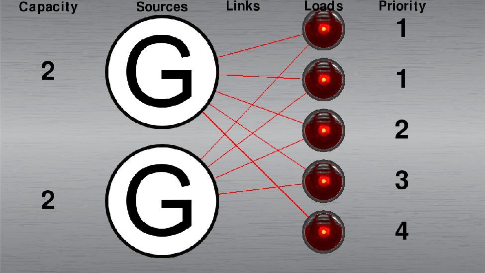
Network example
Ordinarily, the first step is to consider any active links and loads to be inactive, but there are no active loads or links in this initial setup. As the diagram shows, there are two sources that supply five loads. Each of the sources have a capacity of 2, which means that they can each supply up to two loads with power. The loads have priorities of 1, 1, 2, 3, and 4, with 1 being the lowest rank in importance and 4 being the highest. Obviously, with two generators each able to supply at most 2 loads, there is a scarcity of supply. In the best case, we can hope for 4 out of 5 loads to be matched with a generator, with one of the priority 1 loads being left out.Let’s look again at this diagram, but with labels included so we can make our linear programming formulation:
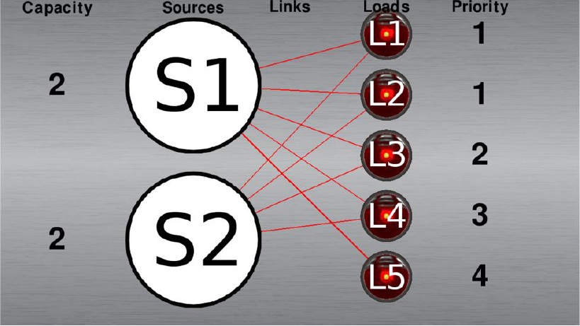
Network example, labeled
These are the names of the links and their incompatibilities with other links in the network:

Example network incompatibilities
The way these links are named is “S->L_N,” where S is the numeric identifier of the source, L is the numeric identifier of the load, and N is the index of link between that particular source and load pair. It is extremely difficult to see in the diagram, but there are two links between S1 and L5. Where more than one link exists, they are displayed on top of each other, and the ones
below are one pixel thicker on each side. It is displayed like this because there may be many links between the same source and load, and this is the best way to fit them all in the same graphic. Incompatibilities between links are just that—two or more links that cannot be activated at the same time as one another. So, for example, if 1->1_1 is to be turned on, then the final solution cannot also contain the link 2->4_1. Where a link is listed as incompatible with another, that other link is also listed as incompatible with it. Incompatibilities are also the reason to include the possibility of multiple links between the same source and load—if a source cannot supply a load through one link because of its incompatibilities with other links, then perhaps it can supply it by another link that to the same load that has a different set of incompatibilities. More about incompatibilities and how they occur is in the next section, Flattening the Distribution Network. For now, we just assume the existence of some arbitrary incompatibilities in the example network. There is some nuance to the priority property of these loads. It is not enough to simply rank them in order of importance. There must also be a decision about what those priority levels mean—are two priority level 1 loads equal to one priority level 2 load? What about two priority level 2 loads against one priority level 3 load? Are they worth a number of points equal to their priority value or does it take two of one level to match the one above it? (Would it take three or would it take four level 1 loads to equal a level 3 load?) To be as realistic as possible, the decision about how to interpret priority levels is this— each priority level unequivocally outclasses all the priority levels below it. No amount of level 1 loads will outmatch a single level 2 load. This is because when loads are ranked by a certain level of importance, we assume it is for good reason. It doesn’t matter how many coffee makers can be supplied on the aircraft if the lights go out, because then no one can see to use them. It doesn’t matter how many coffee makers or lights can be supplied if the navigation system goes out.