Perception in Self-driving

Sensors

Various types of sensors are used for perception in the self-driving industry. Most current solutions rely on either a camera or LIDAR as the main sensor. A camera captures reflections of light passively and stores data as 2D images. In contrast, LIDAR actively emits point laser beams and measures the distance to the point that each laser illuminates by measuring the time of flight. 2D LIDAR systems scan a plane. We are more interested in 3D LIDAR, which scans the 3D space in its field of view (FOV) and stores the reflections as a collection of points in the 3D space, known as a point cloud. Compared to a camera, the intrinsic advantages of LIDAR are that as an active imaging system, it minimizes dependence on light conditions, and secondly, it can scan the 3D space in just one instance. The trade-off is that an industrial grade LIDAR system is much more expensive than a camera.

People often compare LIDAR to RADAR. Similar to LIDAR, RADAR actively emits electromagnetic waves. The frequency band of RADAR is much lower than that of visual light, around which LIDAR operates. Therefore, RADAR waves suffer less attenuation, so RADAR has a longer range. Also, RADAR works more reliably in foggy and smoky environments. On the other hand, LIDAR provides a higher resolution while RADAR’s resolution is too low to be the primary sensor for self-driving.
It is worth noting that almost all current solutions for perception use multimodal sensor fusion, meaning combining information from multiple sensors of different types. For example, Waymo’s fifth-generation self-driving system uses a sensor suite that includes cameras with different ranges, RADARs, 2D LIDARs and one 3D LIDAR [19].

 

Structure of LIDAR

A set of parameters can be used to describe the characteristics of a LIDAR system. The example used here is Velodyne’s HDL-64E. In Table 2.1, the key parameters are listed. The range being 120m is the upper limit of the hardware and can be made smaller as needed. Range accuracy specifies how accurate it can measure the distance to the point of reflection. Number of lines is also widely known as number of channels, which represents the number of laser emitters on the device. When the LIDAR system operates, it rotates the laser emitters horizontally or uses optical designs, such as fixed laser emitters with a rotating reflection panel, to accomplish an equivalent set up. The mainstream configuration of directions of laser emitters, which HDL-64E also uses, is a vertical alignment. Therefore, as the vertical FoV is set, the vertical resolution ∆β is:

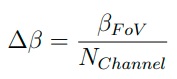
where β_Fov denotes the vertical FoV and N_Channel denotes the number of channels. In the example of HDL-64E, the vertical resolution is 26.9 ^◦/64 = 0.42^◦ . The horizontal FoV of HDL-64E is 360^◦ because it rotates to cover a full circle. However, it is worth noting that not all LIDAR products do the same.

Refresh rate refers to the frequency of horizontal rotation. The frame rate (frames per second, FPS) is embedded in the horizontal resolution. The relationship follows the equation:

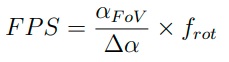
where the α_Fov , ∆_α, and f_rot denote horizontal FoV, horizontal resolution and refresh rate respectively. It is worth noting that α_Fov and f_rot are related by the frequency of sending pulses, which is not provided in [4] and unlisted in Table 2.1. The points per second (PPS) can then be obtained by:

The given points per second is an empirical value. Using equations (2.2) and (2.3), we can calculate the theoretical PPS to be 1,440,000.

 

Point Cloud

A point cloud is a set of points that represents shapes of patterns in space. Specifically in our context, point cloud is the output data format of LIDAR. More generally, point clouds are usually generated by 3D scanning.
Like images and videos, point clouds also have many formats from various organizations and standards. Two examples are Polygon or Stanford triangle format (PLY) and point cloud data (PCD). PLY was set earlier and designed for 3D scanners. PCD
is more recent and created by the author of the popular point cloud library (pcl) [20]. The internal data structure of point clouds is mostly a set of n-tuples. Therefore, less application-specific file formats like binary file (BIN) and comma-separated values (CSV) are also widely used. Point cloud data includes the coordinates and other properties such as intensity and color of each point. Intensity contains information of distance and reflectivity of the surface and color could help visualize segmentation. The availability of point-wise properties and details of the format such as scale and encoding is determined by individual hardware providers.

Point Cloud Processing

Point cloud processing has many tasks. Here we discuss two tasks of our interest: downsampling and registration. Downsampling can reduce the density of a point cloud. Some downsampling algorithms can change the distribution of the point set.
We define a point set P with N points:

The simplest downsampling scheme is downsampling with fixed step size. Assuming r% of the points are kept, the downsampled point set is then:

From the perspective of programming, if the point set is stored in an indexed data structure, we only need to operate on the indices, making this algorithm very fast.
However, the result is heavily affected by the indexing of the original point set and could suffer serious loss of information.

Another downsampling algorithm is called voxel grid downsampling. In the context of point clouds, a voxel can be understood as a box containing points in the 3D space. Given the dimensions of the voxel, the 3D space can be represented by a grid formed by a number of identical voxels. Each point in the point cloud belongs to one of the voxels. Then at most one point is kept in each voxel. There are different methods to select the kept point in each voxel. One is random sampling, which is to randomly select one of the points in the voxel. Another method is to compute and keep the centroid of the points in the voxel. The former method is more efficient while the latter one provides a more accurate description of the original point cloud.
The pseudocode of voxel grid downsampling using the centroid method is shown in Algorithm 1.

The two downsampling algorithms are illustrated in Figure 2.1 using the teapot for comparison. The voxel grid approach introduces much less bias in the distribution of points than the fixed step approach.