An autoencoder is an unsupervised algorithm for generating efficient encodings. The input layer and the target output is typically the same. The layers between decrease and increase in the following fashion:
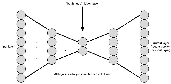
The bottleneck layer is the middle layer with a reduced dimension. The left side of the bottleneck layer is called encoder and the right side is called decoder. An encoder typically reduces the dimension of the data and a decoder increases the dimensions. This combination of encoder and decoder is called an autoencoder. The whole network is trained with reconstruction error. Theoretically, the bottleneck layer can be stored and the original data can be reconstructed by the decoder network. This reduces the dimensions and can be programmed easily, as shown next. Define a convolution, deconvolution, and fully connected layer, using the following code:
def fully_connected_layer(input_layer, units):
    return tf.layers.dense(
        input_layer,
        units=units,
        activation=tf.nn.relu
    )


def convolution_layer(input_layer, filter_size):
    return  tf.layers.conv2d(
        input_layer,
        filters=filter_size,
        kernel_initializer=tf.contrib.layers.xavier_initializer_conv2d(),
        kernel_size=3,
        strides=2
    )


def deconvolution_layer(input_layer, filter_size, activation=tf.nn.relu):
    return tf.layers.conv2d_transpose(
        input_layer,
        filters=filter_size,
        kernel_initializer=tf.contrib.layers.xavier_initializer_conv2d(),
        kernel_size=3,
        activation=activation,
        strides=2
    )
Define the converging encoder with five layers of convolution, as shown in the following code:
input_layer = tf.placeholder(tf.float32, [None, 128, 128, 3])
convolution_layer_1 = convolution_layer(input_layer, 1024)
convolution_layer_2 = convolution_layer(convolution_layer_1, 512)
convolution_layer_3 = convolution_layer(convolution_layer_2, 256)
convolution_layer_4 = convolution_layer(convolution_layer_3, 128)
convolution_layer_5 = convolution_layer(convolution_layer_4, 32)
Compute the bottleneck layer by flattening the fifth convolution layer. The bottleneck layer is again reshaped back fit a convolution layer, as shown here:
convolution_layer_5_flattened = tf.layers.flatten(convolution_layer_5)
bottleneck_layer = fully_connected_layer(convolution_layer_5_flattened, 16)
c5_shape = convolution_layer_5.get_shape().as_list()
c5f_flat_shape = convolution_layer_5_flattened.get_shape().as_list()[1]
fully_connected = fully_connected_layer(bottleneck_layer, c5f_flat_shape)
fully_connected = tf.reshape(fully_connected,
                             [-1, c5_shape[1], c5_shape[2], c5_shape[3]])
Compute the diverging or decoder part that can reconstruct the image, as shown in the following code:
deconvolution_layer_1 = deconvolution_layer(fully_connected, 128)
deconvolution_layer_2 = deconvolution_layer(deconvolution_layer_1, 256)
deconvolution_layer_3 = deconvolution_layer(deconvolution_layer_2, 512)
deconvolution_layer_4 = deconvolution_layer(deconvolution_layer_3, 1024)
deconvolution_layer_5 = deconvolution_layer(deconvolution_layer_4, 3,
                                            activation=tf.nn.tanh)
This network is trained and it quickly converges. The bottleneck layer can be stored when passed with image features. This helps in decreasing the size of the database, which can be used for retrieval. Only the encoder part is needed for indexing the features. Autoencoder is a lossy compression algorithm. It is different from other compression algorithms because it learns the compression pattern from the data. Hence, an autoencoder model is specific to the data. An autoencoder could be combined with t-SNE for a better visualization. The bottleneck layers learned by the autoencoder might not be useful for other tasks. The size of the bottleneck layer can be larger than previous layers. In such a case of diverging and converging connections are sparse autoencoders.