Analytical Solution of Fick’s 2nd law
The rate at which the dye mixes with the water is characterized by determining a dispersion coefficient. The analytical solution for equation 5 when a pulse of mass ’M’ is injected at x=0, the concentration distribution over a cross section of area ‘![]() ’ is given by
’ is given by
(9)
Where C=Concentration (kg/![]() ), M=Mass of dye injected (kg),
), M=Mass of dye injected (kg), ![]() =Cross sectional area of tube (
=Cross sectional area of tube (![]() ), D=Diffusion Coefficient (
), D=Diffusion Coefficient (![]() /s), x=Axial distance (m), t=time (s). This formula characterizes the diffusion of the dye into a solvent medium. The rate at which a dye mixes with water in an oscillating flow is established by substituting the diffusion coefficient in equation 9 with a dispersion coefficient,
/s), x=Axial distance (m), t=time (s). This formula characterizes the diffusion of the dye into a solvent medium. The rate at which a dye mixes with water in an oscillating flow is established by substituting the diffusion coefficient in equation 9 with a dispersion coefficient,  .
.
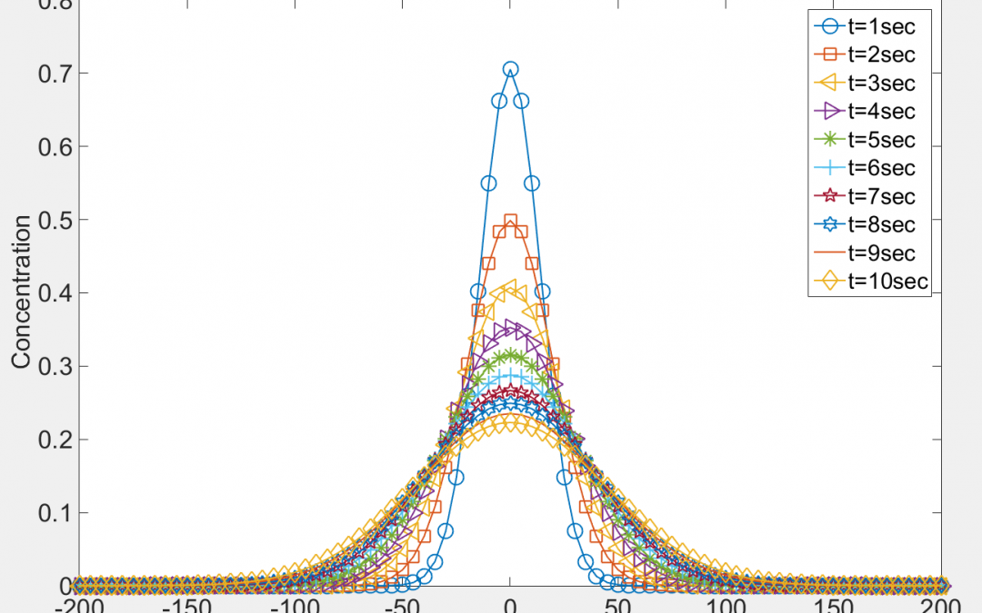
In order to demonstrate the nature of the concentration curves, Equation 9 is evaluated by considering arbitrary values of variables M, ![]() and x. The value of is arbitrarily considered 100, and the value of t is considered from 1 to 10 in steps of 1. The resulting concentration values are plotted vs. distance for different time steps in 8 shows the decaying concentration profiles as the dye diffuses over time.
and x. The value of is arbitrarily considered 100, and the value of t is considered from 1 to 10 in steps of 1. The resulting concentration values are plotted vs. distance for different time steps in 8 shows the decaying concentration profiles as the dye diffuses over time.
Figure 8: Concentration vs. Distance at different times. Concentration curves are plotted by solving equation 6 with arbitrary values. Each curve represents the concentration at a time step.
A plot of concentration vs. distance at a particular time step is a Gaussian function. The Area Parameter (AP) for a gaussian curve is the area under the curve divided by the peak concentration of the curve. The values of AP for each concentration curve shown in Fig.8 increase with time. At time t=0, Equation 9 is unsolvable because of division by zero. As time tends to zero, the AP value tends to 1. Hence the AP value at t=0 is set to 1. If is kept constant, changing the values of variables M, Ac, C and x have no effect on the AP value for a particular time step. However, changing the value of changes the AP values. Fig.9 shows AP vs. Time for ranging from 100 to 200 in steps of 10. It is observed that a plot of AP at different time steps for a specific has its unique locus. The AP curve corresponding to Fig.8 is represented by =100 in Fig.9. Hence the AP values over time are characteristic of and can be used to determine experimentally.
Figure 9: AP vs. Time for different Deff. AP values are plotted over time for different Deff values. Each AP curve has a unique locus for a specific value of Deff. These curves can be used to obtain values of Deff for experiments. AP values corresponding to Deff=100, represents AP values for concentration curves shown in Fig.9
AP values obtained by solving equation 9 are hereby referred to as Analytical AP.