
Global Positioning System
The global positioning system (GPS) is a navigation system supported by satellites that provides location information for objects on or near the surface of the earth. The navigation satellite timing and ranging (NAVSTAR) GPS has been functioning since 1993 and was developed by the United States Department of Defense. The GPS is one of the most important technologies that allows the functioning of UAS, giving them spatial localization.
In this section we explain brie y how the sensing works in GPS systems and we present a GPS model appropriate for simulation.
The most important element in the GPS system is the 24 satellites that orbit continuously around the earth at an altitude of 20,180 km. The constellation of the satellites orbits is congured so that any location on the surface of the earth can be observed by at least four satellites all the time. It is common knowledge that with one range measurement is possible to locate a point in a line. With two range measurements a point on a plane and with three range measurements, a point on a 3-D surface. This explains the need for three of the four satellites. But the last one comes from clock synchronization errors between the satellites and the receiver. Therefore, with four independent pseudo-range measurements, there exists a system of four nonlinear equations which yield to the solution of the four variables of interest: latitude, longitude, altitude and receiver clock time offset.
GPS Measurement Error Model
The two factors that affect the precision of a GPS position measurement are the accuracy of the satellite pseudo-range measurements and the conguration of the satellites from which these pseudo-measurements are taken. The rst factor is impacted by errors in the time of ight for each satellite. Where the second one is considered in a term called dilution of precision (DOP).
Ephemeris Data
The satellite ephemeris gives the position of the satellite in the sky at a given time. The position of the GPS receiver is calculated using measurement ranges with respect to satellites. To determine this position, we are required to know the locations of the satellites in the rst place. Ephemeris errors in the measurements exists because of the inaccuracies in the transmitted orbital satellite location. Common errors vary from 1 to 5 m.
Satellite Clock
The atomic clocks used in GPS satellites are made of cesium and rubidium. These clocks can drift about 10 ns a day. This translates to an error of 3.5 m. But their clocks are synchronized twice a day, therefore leading to an approximately 1.75 m error.
Ionosphere
This is the topmost layer of the atmosphere of the earth and consists of a shell of electrons and electrically charged atoms and molecules that surround the earth. This particles can delay the transmission of GPS signals. Even though the GPS receivers compensate for this delay, variations in the speed of light along this atmosphere’s layer, is the biggest cause of
GPS measurement errors, which contributes to approximately 2 to 5 m.
Troposphere
The troposphere is the lowest portion of the atmosphere containing approximately 80% of the atmosphere’s mass and is located at an altitude of 7 to 20 km. Most of the weather phenomena occurs in this region. This produces variations in the speed of light and consequently in the time of ight and pseudo-range estimates. These variations introduces errors in the GPS measurements of about 1 m.
Multipath Reception
Multipath errors occur when re ected signals are received by the GPS receiver, mixing with the real signal. Big surfaces as large buildings or structures increases this error. Normally this error source contributes to 1 m of variation in the GPS measurement.
Receiver Measurement
This error is caused by the implicit limits with which the time of the satellite signal can be calculated. Modern receivers errors for this source is less than 0.5 m.
The pseudo-range error sources described previously are considered statistically uncorrelated and we can use the root sum of squares to add them. The addition of all of these error sources is called the user-equivalent range error. Parkinson, et al.characterized these errors as a combination of slowly varying biases and random noise.
Transient Characteristic of GPS Positioning Error
For simulation purposes we are required to know the dynamic characteristics of the GPS error. According to, the dynamic model that describes the GPS error is a Gauss- Markov process which is modeled by
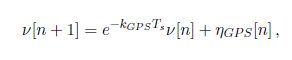
1
where is the error being modeled,
is zero-mean Gaussian white noise,
is the time constant of the process, and
is the sample time. An appropriate model for simulation of GPS measurements is given by
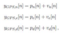
2,3,4
where ,
, and pd are the position coordinates in the local tangent plane or the North East Down coordinate system, and n is the time step of the measurement. Usually the GPS receivers used by small UAV have a measurement frequency of 1 to 4 Hz.
GPS Velocity Measurements
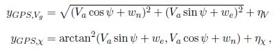
Using the Doppler Effect, which is the changes in frequency of a wave for an observer moving relative to its source, the speed of the GPS receiver can be estimated. This approximation has a standard deviation of 0.01 to 0.05 m/s. Modern GPS receivers usually provide more than just the position and also include the velocity of the receiver, horizontal ground speed and course angle. The last two are calculated from the north and east velocity components as
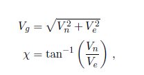
5,6
where
![]()
Using uncertainty analysis as in, the uncertainty in ground speed and course measurements can be approximated as
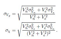
If the uncertainty in the north and east axis have the same magnitude , these formulas simplify a

7,8
In these expressions we can observe that the uncertainty in the course measurements increases with the inverse of the ground speed with high speeds yielding small errors and low velocity creating big errors. The reason for this behavior is because the course angle is only dened for moving objects. The ground speed and the course angle measurements of the GPS receiver can be modeled parting from (5)-(6) and (7)-(8)
9,10
where and
are zero-mean Gaussian processes with variances
and
GPS Smoothing
In this section we present an algorithm that estimates the position, ground speed, course, wind speed and heading of a xed wing aircraft. Assuming that the ight path angle ( ) is zero, the position can be expressed as
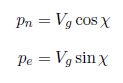
where is the course angle of the UAS. To get the variation of the ground speed we must differentiate (5) getting
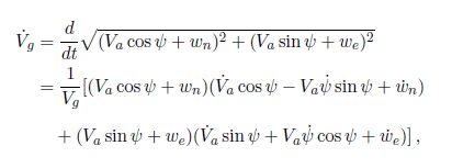
where and
are the wind speed in the north and the east direction respectively, and
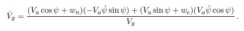
is the air velocity. If we assume that the wind speed and airspeed are constant the evolution of the ground speed simplies to
On the other hand, the evolution of is described as
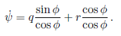
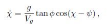 and the dynamic of
 is given by
 The nonlinear propagation model is given by
 , where x is the state and is dened as
, and u is the input expressed as
, and x is dened as
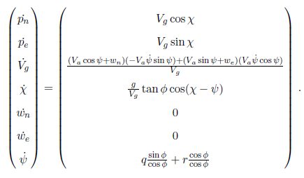
11.
The Jacobian matrix, obtained by taking partial derivatives of the propagation model x= f(x; u) with respect to x, is expressed as
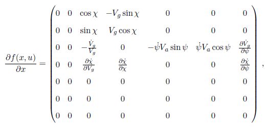
12
where
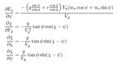
The input u is composed by the north position, east position, ground speed, and course supplied by the GPS receiver.
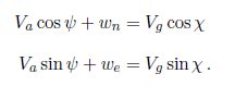
For measurements, we use the GPS signals for north and east position, ground speed and course. Due to the coupling of the states, we require the triangle relationship given by 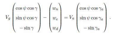 If we assume that
 =
= 0, the down component is discarded, and we are left with
Using these equations we can dene the pseudo measurements as
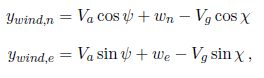
The consequent measurement model is expressed as
![]()
where = (
),
, and
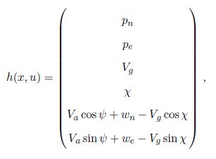
13
And the Jacobian, obtained by taking partial derivatives of the measurement model with respect to x, is given by
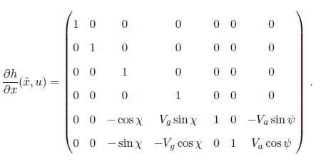
14
The estimation of and
, are going to be calculated using two algorithms called the extended Kalman lter (EKF) and the delayed extended Kalman lter (DEKF).

GPS