Introduction to Array Operations in MATLAB
In the meeting with the MATLAB environment, we said that we can use MATLAB as a calculator. When you read the word calculator, what kind of calculator came to your mind? Simple calculators for shopkeepers or engineering calculators with a button? We have to say that MATLAB is a complex engineering calculator with a sea of different possibilities. In this session, we want to show you a corner of these features.
Addition and subtraction of matrices and vectors in MATLAB
Perhaps the title of the simplest mathematical operation can be attributed to addition and subtraction. You have already seen that in MATLAB you can easily add or subtract two numbers together. look:
>> 8 - 2
ans =
    6

>> 4 + 5
ans =
    9
In the same way, arrays can be added or subtracted. We know from mathematics that arrays must have the same dimensions to add or subtract. Make sure you always follow this simple but important point. Define two vectors called a1 and a2. Make vectors of any size you like. We considered the length of the vector to be 5. Then add these vectors once and subtract once:
>> a1 = randi(10, 1, 5)
a1 =
     9   10   2   10   7

>> a2 = randi(10, 1, 5)
a2 =
     1   3   6   10   10

>> a1 + a2
ans =
     10   13   8   20   17

>> a1 - a2
ans =
     8   7   -4   0   -3
Well, we could easily add and subtract two equal vectors. Matrices can be added and subtracted in the same way. Let’s define two matrices called b1 and b2 with dimensions of 2 in 3. Then add and subtract them:
>> b1 = randi(10, 2, 3)
b1 =
    2    10   9
    10   5    2

>> b2 = randi(10, 2, 3)
b2 =
    5   8   7
    10  10  1

>> b1 - b2
ans =
    -3    2   2
     0   -5   1

>> b1 + b2
ans =
    7    18   16
    20   15    3
Now, what happens if the dimensions of the two matrices are not equal? For example, let’s add the vector a1 to the matrix b1:
>> a1 + b1
Matrix dimensions must agree.
You can see that MATLAB has given an error. This error says: Matrix dimensions must agree. That is, the dimensions of the matrices must be equal. So if you encounter such an error, know that your matrices are not the same size. Well, it’s pretty clear. Subtraction and subtraction are done in two arrays (matrix or vector). If they are not the same size, some elements do not have a corresponding value.
Note: This is the first time that we have shown you an error in MATLAB during these sessions. You see, when we translate an error into Persian, it is easily meaningful. We have seen very, very much that students stop working when they see the slightest mistake. Or open Telegram and send error screenshots to all member groups. Or worse, they do not send screenshots and only announce in the group that a MATLAB specialist will come to help! Beloved, believe me, debugging is not a difficult task. Read the error and then translate it. If you do not find what you are looking for then just ask. That is, copy the red error above into Google. A site like StackOverflow usually answers over 90% of these questions.
Our forum contains most errors, https://matlab1.com/forum/index.php
Matrices and vectors can be added or subtracted with a scalar (one number). Well, you might say that matrices and vectors are not the same size as a scalar and that addition or subtraction is meaningless. But in practice, this is not the case. If in MATLAB we add a matrix or vector with a scalar, that scalar will be added with all the elements. The same is true for subtraction. That scalar will be deducted from all assets. Now to make it clear to you, add 4 to a1 and subtract 1 from b2:
>> a1
a1 =
    9   10   2   10   7
>> a1 + 4
ans =
    13   14   6   14   11

>> b2 =
    5   8   7
   10   10  1
>> b2 - 1
ans =
    4   7   6
    9   9   0
Notice that 4 units were added to all a1 devices. Also, one unit of all b2 devices is reduced.
Multiplication in MATLAB
Multiplication of numbers in MATLAB can also be done easily with the * operator. For example, to multiply two numbers, it is enough to write:
>> 4 * 6
ans =
     24
Multiplications and matrices, however, have a point. There are three modes for multiplying matrices and vectors: matrix multiplication, multiplication by multiplication, and scalar multiplication by a matrix or vector. In the following, we will examine each of these cases.
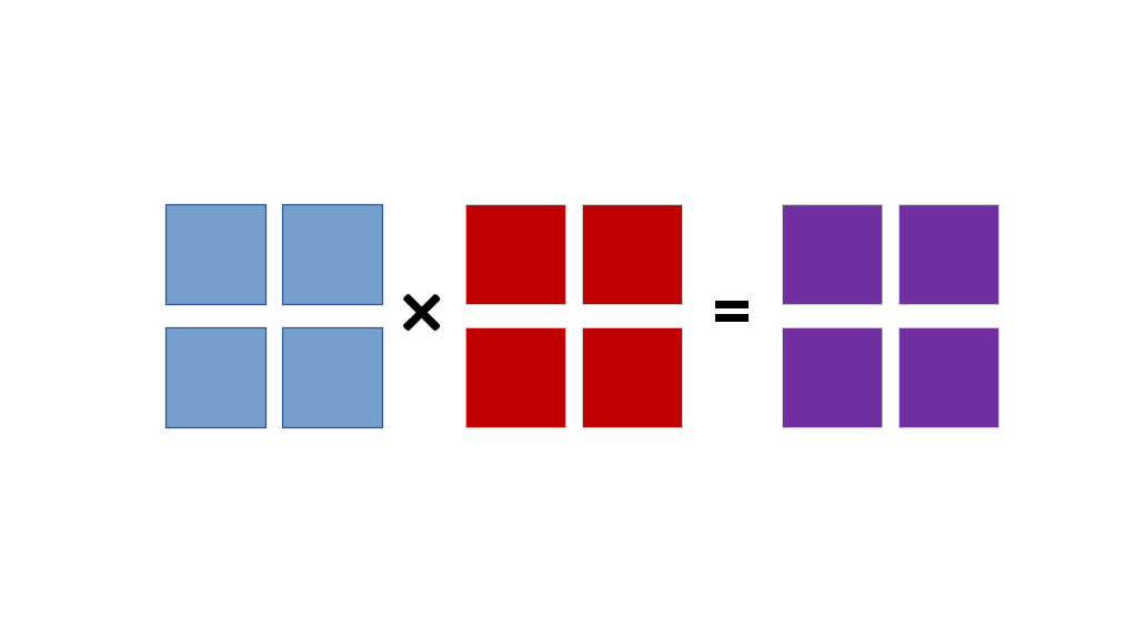
1- Matrix multiplication in MATLAB
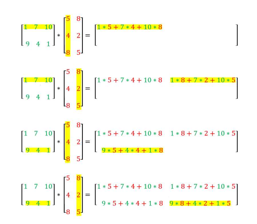
Multiplication matrices
Matrix multiplication is shown in the image above. In mathematics, we can not multiply both vectors or matrices we want. We can multiply vectors or matrices whose dimensions are compatible. What does it mean? Pay attention to the word compatible. We did not say that the dimensions are equal, we said that it is compatible… that is, the number of columns of the first matrix is equal to the number of rows of the second matrix. That is, if the dimensions of the first matrix are m × n, the dimensions of the second matrix must be n × k.
The b1 matrix we defined earlier was 3 × 2. We want to define a new matrix and multiply by b1. According to the law we said, how many rows should the new matrix have? Yes, it should have 3 lines. Consider the number of columns, for example, 4. Multiply the name of the new matrix by c then b by b1:
>> c = randi(10, 3, 4)
c =
    9    8   7   1
    10   8   2   3
    7    4   8   1

>> b1 * c
ans =
    181   132   106   41
    154   128   96    27
You can see that the two matrices are multiplied. You may want to be sure of the rule we used to multiply matrices. What do you think would happen if we multiplied b1 by b2? The dimensions of both are 3 × 2. Let’s try:
Error using *
Incorrect dimensions for matrix multiplication. Check that the number of columns in the
 first matrix matches the number of rows in the second matrix. To perform elementwise
 multiplication, use '.*'.
MATLAB tells you to check that the number of columns in the first matrix is equal to the number of rows in the second matrix. If you are familiar with the multiplication of matrices in mathematics, the law of multiplication of matrices will be obvious to you. But if you are not familiar with the multiplication of matrices, I want you to learn as soon as possible! Because knowing the theory is also important and necessary in coding.
The same rule applies to multipliers. A column vector of length m (i.e., dimensions m in 1) can be multiplied by a line vector of length k (i.e., dimensions 1 in k). A line vector of length n (i.e., dimensions 1 in n) can be multiplied by a column vector of length n (i.e., dimensions n in 1) or a matrix of dimensions n in k.
2- Multiplication by line in MATLAB
Multiply by element-wise means that arrays are multiplied by each other. Exactly the same addition and subtraction as we said, the following image shows an example of this type of multiplication:
In multiplication, the multiplications are multiplied peer-to-peer. It is clear that in this type of multiplication, the dimensions of the arrays must be equal. In mathematics, this type of matrix multiplication may not be important. But when dealing with data, we often need this type of multiplication. Multiply data by data in MATLAB with the operator *. It can be done. Note that there is a dot next to the * sign. In general, when we put a dot next to an operator, we mean operation side by side. So for example, multiply b1 and b2 side by side:
>> b1 .* b2
ans =
  10   80  63
  100  50  2
You see using the *. sign. Instead of * not only did he not make a mistake, but the two matrices were multiplied by the method. You can see that the dimensions of the output matrix are equal to the input matrix.
3- Scalar multiplication in array in MATLAB
In addition and subtraction, you can multiply all the elements of an array in one scalar. For example:
>> a1 * 3
ans =
     27   30   6   30   21

>> b1 * 2
ans =
     4    20    18
     20   10    4
Division in MATLAB
Dividing numbers in MATLAB with the / operator can be done. For example:
>> 7 / 3
ans =
    2.3333
Like multiplication, there are three modes for dividing matrices and vectors: matrix division, array-to-array division, and scalar division in a matrix or vector. In the following, we will examine each of these cases.
1- Matrix division
Divisions for matrices and vectors are not defined in mathematics. We do not have something called dividing a matrix by a matrix. So what if we write in MATLAB, for example, b1 / b2? Do we get an error? Let’s see:
>> b1 / b2
ans =
    1.4584   -0.3522

    0.0089   0.7501
So now the question arises that if there is no division of two matrices, then what is this ?! In mathematics to solve the equation 3x = 6 we quickly divide 6 by 3 and x becomes 2! But getting x in the matrix equation Ax = C is not so simple. In this equation, we cannot divide C by A. Because there is no division of two definition matrices at all! So how is this equation solved? This equation is solved as follows:
XA = C
XAA–1 = CA–1
XI = CA–1
X = CA–1
X = C / A
In MATLAB, exactly the same result is returned. That is, the mathematical expression CA-1 is equivalent to the same C / A in MATLAB. Wasn’t it interesting?
Exercise 1: If we use the equation AX = C instead of /! Why? Solve the same as above …
AX = C
A–1AX = A–1C
IX = A–1C
X = A–1C = A / C
2. Divide element to element
Just like multiplication, in the division of a particle into a particle, the elements of two matrices or peer-to-peer vectors are divided. In MATLAB to perform partition to partition from operator /. Is used. Note that the dimensions of the two matrices must be equal when dividing the flow. For example, suppose we want to divide two matrices b1 and b2 by the following:
>> b1 ./ b2
ans =
    0.4000   1.2500   1.2857
    1.0000   0.5000   2.0000
Note that here, too, the dimensions of the output are exactly the same as the input matrices.
3- Dividing the array by the scalar
In MATLAB, with the / operator, a matrix or vector can be divided into a scalar. For example, suppose we want to divide the vector a1 by 6. will have:
>> a1 / 6
ans =
    1.5000   1.6667   0.3333   1.6667   1.1667
Is it clear anymore? All devices a1 are divided by number 6.
Power in MATLAB
The ^ symbol is used to enable a number in MATLAB. for example:
>> 2 ^ 5
ans =
 32
Enabling Arrays But What Does It Mean? That is, what is a matrix to the power of, say, 2? In MATLAB, a matrix to the power of 2 means multiplying the matrix by itself. What about higher powers? For example, what does a matrix with the power of 4 mean? In MATLAB, multiply a matrix by itself 4 times. Now, for example, let’s increase b1 to the power of 3:
>> b1 ^ 3
Error using ^ (line 51)
Incorrect dimensions for raising a matrix to a power. Check that the matrix is square
 and the power is a scalar. To perform elementwise matrix powers, use '.^'.
We made a mistake! This error says that the dimensions of the matrices do not read together. We forgot an important point. Weren’t the first columns equal to the second rows if we multiplied the dumatrix? Well, our b1 matrix was 2 by 3. That it cannot be multiplied in itself. Therefore, we can only enable matrices in MATLAB that have the same number of rows and columns. That is, be a square matrix. So the condition for using the operator که is that our matrix is square. Obviously, we can not power vectors either.
Like multiplication and division, the operator ^. Power to power. For example, if we want to increase the same b1 from power to power by 3, we must write:
>> b1 .^ 3
ans =
 8 1000 729
 1000 125 8
You can see that each of the b1 devices has reached the power of 3.
as
